Detector geometry reference
The AGIPD and LPD detectors are made up of several sensor modules, from which separate streams of data are recorded. Inspecting or processing data from these detectors therefore depends on knowing how the modules are arranged. EXtra-geom handles this information.
All the coordinates used in this module are from the detector centre. This should be roughly where the beam passes through the detector. They follow the standard European XFEL axis orientations, with x increasing to the left (looking along the beam), and y increasing upwards.
This module includes
position_modules_interpolate() to
assemble data into a single 2D array with pixel splitting, conserving total
signal (using pyFAI’s
[Distortion](https://pyfai.readthedocs.io/en/stable/usage/tutorial/Detector/Distortion/Distortion.html)
module). For accurate analysis, it’s still best to use tools that can process
geometry without relying on assembled images, both for performance and
correctness. However, this method can be useful for previewing data, or for
processing with tools that require images of the complete detector.
position_modules() gives a faster but
less accurate geometry assembly snapping detector pixels to a regular grid.
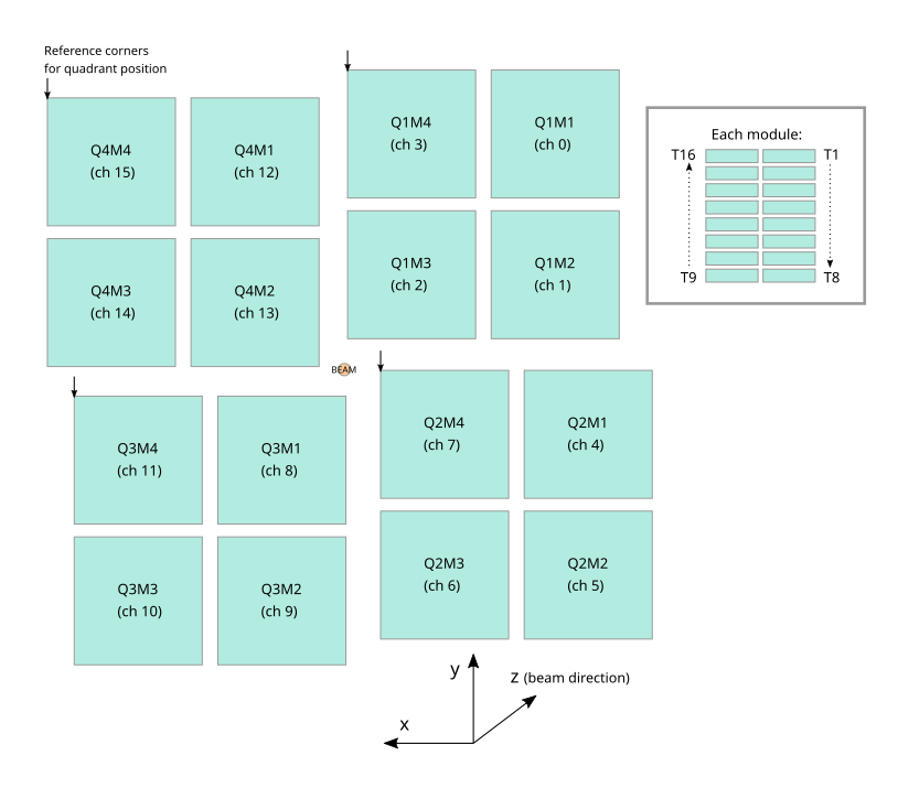
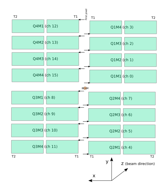
AGIPD-1M
AGIPD-1M consists of 16 modules of 512×128 pixels each. Each module is further subdivided into 8 tiles. The layout of tiles within a module is fixed by the manufacturing process, but this geometry code works with a position for each tile.
The approximate layout of AGIPD-1M, in a front view (looking along the beam).
- class extra_geom.AGIPD_1MGeometry(modules, filename='No file', metadata=None)
Detector layout for AGIPD-1M
The coordinates used in this class are 3D (x, y, z), and represent metres.
You won’t normally instantiate this class directly: use one of the constructor class methods to create or load a geometry.
- classmethod from_quad_positions(quad_pos, asic_gap=2, panel_gap=29, unit=0.0002)
Generate an AGIPD-1M geometry from quadrant positions.
This produces an idealised geometry, assuming all modules are perfectly flat, aligned and equally spaced within their quadrant.
The quadrant positions are given in pixel units, referring to the first pixel of the first module in each quadrant, corresponding to data channels 0, 4, 8 and 12.
The origin of the coordinates is in the centre of the detector. Coordinates increase upwards and to the left (looking along the beam).
To give positions in units other than pixels, pass the unit parameter as the length of the unit in metres. E.g.
unit=1e-3means the coordinates are in millimetres.
- classmethod from_crystfel_geom(filename)
Read a CrystFEL format (.geom) geometry file.
Returns a new geometry object.
- classmethod example()
Create an example geometry (useful for quick visualization).
- offset(shift, *, modules=slice(None, None, None), tiles=slice(None, None, None))
Move part or all of the detector, making a new geometry.
By default, this moves all modules & tiles. To move the centre down in the image, move the whole geometry up relative to it.
Returns a new geometry object of the same type.
# Move the whole geometry up 2 mm (relative to the beam)
geom2 = geom.offset((0, 2e-3))

# Move quadrant 1 (modules 0, 1, 2, 3) up 2 mm
geom2 = geom.offset((0, 2e-3), modules=np.s_[0:4])

# Move each module by a separate amount
shifts = np.zeros((16, 3))
shifts[5] = (0, 2e-3, 0)    # x, y, z for individual modules
shifts[10] = (0, -1e-3, 0)
geom2 = geom.offset(shifts)
- Parameters:
shift (numpy.ndarray or tuple) – (x, y) or (x, y, z) shift to apply in metres. Can be a single shift for all selected modules, a 2D array with a shift per module, or a 3D array with a shift per tile (
arr[module, tile, xyz]).modules (slice) – Select modules to move; defaults to all modules. Like all Python slicing, the end number is excluded, so
np.s_[:4]moves modules 0, 1, 2, 3.tiles (slice) – Select tiles to move within each module; defaults to all tiles.
- rotate(angles, center=None, modules=slice(None, None, None), tiles=slice(None, None, None), degrees=True)
Rotate part or all of the detector, making a new geometry.
The rotation is defined by composition of rotations about the axes of the coordinate system (https://en.wikipedia.org/wiki/Euler_angles), i.e. a rotation around the z axis rotates the xy (detector) plan. We use the right-hand rule, xy being the detector plan with z increasing looking toward the detector front plan, x increasing to the left, y increasing to the top. Positive rotations are clockwise.
In other words:
Positive x angles tilt the top edge of the detector backwards, away from the source
Positive y angles tilt the right-hand edge (looking along the beam) away from the source
Positive z angles turn the detector clockwise (looking along the beam)
By default, this rotates all modules & tiles. Returns a new geometry object of the same type.
# Rotate the whole geometry by 90 degree in the xy plan
geom2 = geom.rotate((0, 0, 90))

# Move the tile 0 in the module 0 around its center by 90 degrees
geom2 = geom.rotate((0, 0, 90), modules=np.s_[:1], tiles=np.s_[:1])

# Rotate each module by a separate amount
rotate = np.zeros((16, 3))
rotate[5] = (3, 5, 1)  # x, y, z for individual modules
rotate[10] = (0, -2, 1)
geom2 = geom.rotate(rotate)
- Parameters:
angles (np.array or tuple) – (x, y, z) rotations to apply in degree. Can be a single rotation for all selected modules, a 2D array with a rotation per module, or a 3D array with a rotation per tile (
arr[module, tile, xyz]).center (np.array or tuple) – center of rotation. Shape must match angles.shape. If set to None (default), the rotation center is set to: * all modules: center of the detector * selected modules: centers of modules * selected tiles: centers of tiles
modules (slice) – Select modules to rotate; defaults to all modules.
tiles (slice) – Select tiles to move within each module; defaults to all tiles.
degrees (bool) – If True (default), angles are in degrees. If False, angles are in radians.
- quad_positions()
Retrieve the coordinates of the first pixel in each quadrant
The coordinates returned are 2D and in pixel units, compatible with
from_quad_positions().
- write_crystfel_geom(filename, *, data_path=None, mask_path=None, dims=('frame', 'modno', 'ss', 'fs'), nquads=None, adu_per_ev=None, clen=None, photon_energy=None)
Write this geometry to a CrystFEL format (.geom) geometry file.
If the geometry was read from a
.geomfile byfrom_crystfel_geom(), some of the optional fields will be filled from metadata if not specified.- Parameters:
filename (str) – Filename of the geometry file to write.
data_path (str) – Path to the group that contains the data array in the hdf5 file. Default:
'/entry_1/instrument_1/detector_1/data'.mask_path (str) – Path to the group that contains the mask array in the hdf5 file.
dims (tuple) – Dimensions of the data. Extra dimensions, except for the defaults, should be added by their index, e.g. (‘frame’, ‘modno’, 0, ‘ss’, ‘fs’) for raw data. Default:
('frame', 'modno', 'ss', 'fs'). Note: the dimensions must contain frame, ss, fs.adu_per_ev (float) – ADU (analog digital units) per electron volt for the considered detector.
clen (float) – Distance between sample and detector in meters
photon_energy (float) – Beam wave length in eV
- get_pixel_positions(centre=True)
Get the physical coordinates of each pixel in the detector
The output is an array with shape like the data, with an extra dimension of length 3 to hold (x, y, z) coordinates. Coordinates are in metres.
If centre=True, the coordinates are calculated for the centre of each pixel. If not, the coordinates are for the first corner of the pixel (the one nearest the [0, 0] corner of the tile in data space).
- to_distortion_array(allow_negative_xy=False)
Return distortion matrix for AGIPD detector, suitable for pyFAI.
- Parameters:
allow_negative_xy (bool) – If False (default), shift the origin so no x or y coordinates are negative. If True, the origin is the detector centre.
- Returns:
out – Array of float 32 with shape (8192, 128, 4, 3). The dimensions mean:
8192 = 16 modules * 512 pixels (slow scan axis)
128 pixels (fast scan axis)
4 corners of each pixel
3 numbers for z, y, x
- Return type:
ndarray
- to_pyfai_detector(**kwargs)
Make a PyFAI detector object for this detector
You can use PyFAI to azimuthally integrate detector images around the centre point of the geometry. The detector object holds the positions of all the pixels. See the examples for how to use this.
- plot_data(data, *, axis_units='px', frontview=True, ax=None, figsize=None, colorbar=True, interpolate=False, **kwargs)
Plot data from the detector using this geometry.
This approximates or interpolate (with interpolate=True) the geometry to align all pixels to a 2D grid.
Returns a matplotlib axes object.
This method was previously called
plot_data_fast, and can still be called with that name.- Parameters:
data (ndarray) – Should have exactly 3 dimensions, for the modules, then the slow scan and fast scan pixel dimensions.
axis_units (str) – Show the detector scale in pixels (‘px’) or metres (‘m’).
frontview (bool) – If True (the default), x increases to the left, as if you were looking along the beam. False gives a ‘looking into the beam’ view.
ax (~matplotlib.axes.Axes object, optional) – Axes that will be used to draw the image. If None is given (default) a new axes object will be created.
figsize (tuple) – Size of the figure (width, height) in inches to be drawn (default: (10, 10))
colorbar (bool, dict) – Draw colobar with default values (if boolean is given). Colorbar appearance can be controlled by passing a dictionary of properties.
interpolate (bool) – If True, use interpolation when drawing the image.
kwargs – Additional keyword arguments passed to ~matplotlib.imshow
- position_modules(data, out=None, threadpool=None)
Assemble data from this detector according to where the pixels are.
This approximates the geometry to align all pixels to a 2D grid.
This method was previously called
position_modules_fast, and can still be called with that name.- Parameters:
data (ndarray or xarray.DataArray) – The last three dimensions should match the modules, then the slow scan and fast scan pixel dimensions. If an xarray labelled array is given, it must have a ‘module’ dimension.
out (ndarray, optional) – An output array to assemble the image into. By default, a new array is allocated. Use
output_array_for_position()to create a suitable array. If an array is passed in, it must match the dtype of the data and the shape of the array that would have been allocated. Parts of the array not covered by detector tiles are not overwritten. In general, you can reuse an output array if you are assembling similar pulses or pulse trains with the same geometry.threadpool (concurrent.futures.ThreadPoolExecutor, optional) – If passed, parallelise copying data into the output image. By default, data for different tiles are copied serially. For a single 1 MPx image, the default appears to be faster, but for assembling a stack of several images at once, multithreading can help.
- Returns:
out (ndarray) – Array with one dimension fewer than the input. The last two dimensions represent pixel y and x in the detector space.
centre (ndarray) – (y, x) pixel location of the detector centre in this geometry.
- output_array_for_position(extra_shape=(), dtype=<class 'numpy.float32'>)
Make an empty output array to use with position_modules
You can speed up assembling images by reusing the same output array: call this once, and then pass the array as the
out=parameter toposition_modules(). By default, it allocates a new array on each call, which can be slow.- Parameters:
extra_shape (tuple, optional) – By default, a 2D output array is generated, to assemble a single detector image. If you are assembling multiple pulses at once, pass
extra_shape=(nframes,)to get a 3D output array.dtype (optional (Default: np.float32))
- position_modules_symmetric(data, out=None, threadpool=None)
Assemble data with the centre in the middle of the output array.
The assembly process is the same as
position_modules(), aligning each module to a single pixel grid. But this makes the output array symmetric, with the centre at (height // 2, width // 2).- Parameters:
data (ndarray or xarray.DataArray) – The last three dimensions should match the modules, then the slow scan and fast scan pixel dimensions. If an xarray labelled array is given, it must have a ‘module’ dimension.
out (ndarray, optional) – An output array to assemble the image into. By default, a new array is created at the minimum size to allow symmetric assembly. If an array is passed in, its last two dimensions must be at least this size.
threadpool (concurrent.futures.ThreadPoolExecutor, optional) – If passed, parallelise copying data into the output image. See
position_modules()for details.
- Returns:
out – Array with one dimension fewer than the input. The last two dimensions represent pixel y and x in the detector space.
- Return type:
ndarray
- position_modules_interpolate(data, *, oversample: int = 1, output_pixel_size=None, resize: bool = True, method: str = 'LUT', empty=nan, device: str | None = None, dis_kwargs: dict | None = None)
Assemble data onto a regular grid using pixel-splitting.
This uses pyFAI’s distortion correction machinery to produce an output image corrected from spatial distortion.
- Parameters:
data (ndarray or xarray.DataArray) – Detector data shaped like
expected_data_shape, optionally with extra leading dimensions.oversample (int) – Subdivide output pixels by this factor in each dimension.
output_pixel_size (float or (float, float), optional) – Output pixel size in metres as
(x, y). If omitted, defaults to the detector pixel size.resize (bool) – If True (default), expand the output array to include all pixels so total signal is preserved.
method (str) – pyFAI distortion backend, e.g. “CSR” or “LUT” (default).
empty (float) – Value for empty output pixels.
device (str, optional) – Name of the device: None for OpenMP, “cpu” or “gpu” or the id of the OpenCL device a 2-tuple of integer.
dis_kwargs (dict, optional) – Extra arguments passed to pyFAI’s
Distortion.correct_ng().
- Returns:
out (ndarray) – Assembled image array (counts), with the module dimension removed.
centre (ndarray) – (y, x) output pixel coordinates of the detector centre.
- inspect(axis_units='px', frontview=True)
Plot the 2D layout of this detector geometry.
Returns a matplotlib Axes object.
- compare(other, scale=1.0)
Show a comparison of this geometry with another in a 2D plot.
This shows the current geometry like
inspect(), with the addition of arrows showing how each panel is shifted in the other geometry.- Parameters:
other (DetectorGeometryBase) – A second geometry object to compare with this one. It should be for the same kind of detector.
scale (float) – Scale the arrows showing the difference in positions. This is useful to show small differences clearly.
- data_coords_to_positions(module_no, slow_scan, fast_scan)
Convert data array coordinates to physical positions
Data array coordinates are how you might refer to a pixel in an array of detector data: module number, and indices in the slow-scan and fast-scan directions. But coordinates in the two pixel dimensions aren’t necessarily integers, e.g. if they refer to the centre of a peak.
module_no, fast_scan and slow_scan should all be numpy arrays of the same shape. module_no should hold integers, starting from 0, so 0: Q1M1, 1: Q1M2, etc.
slow_scan and fast_scan describe positions within that module. They may hold floats for sub-pixel positions. In both, 0.5 is the centre of the first pixel.
Returns an array of similar shape with an extra dimension of length 3, for (x, y, z) coordinates in metres.
See also
Converting array coordinates to physical positions demonstrates using this method.
- extra_geom.agipd_asic_seams()
Make a boolean array marking the double-width pixels in an AGIPD module
This returns a (512, 128) array with False for normal (square) pixels, and True for the 400 x 200 µm pixels at the horizontal joins between ASICs.
See Making data masks for an illustration of this.
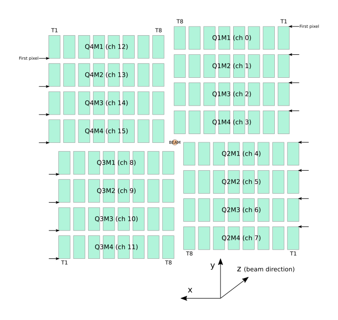
AGIPD-500K2G
AGIPD-500K2G consists of 8 modules of 512×128 pixels each. Each module is further subdivided into 8 tiles. The layout of tiles within a module is fixed by the manufacturing process, but this geometry code works with a position for each tile.
The approximate layout of AGIPD-500K2G, in a front view (looking along the beam).
- class extra_geom.AGIPD_500K2GGeometry(modules, filename='No file', metadata=None)
Detector layout for AGIPD-500k
The coordinates used in this class are 3D (x, y, z), and represent metres.
You won’t normally instantiate this class directly: use one of the constructor class methods to create or load a geometry.
- classmethod from_origin(origin=(0, 0), asic_gap=None, panel_gap=None, unit=0.0002)
Generate an AGIPD-500K2G geometry from origin position.
This produces an idealised geometry, assuming all modules are perfectly flat, aligned and equally spaced within the detector.
The default origin (0, 0) of the coordinates is the bottom-right corner of the detector. If another coordinate is given as the origin, it is relative to the bottom-right corner. Coordinates increase upwards and to the left (looking along the beam).
The default gaps (when set to None) are: asic_gap=2 and panel_gap=(16, 30) pixels.
To give positions in units other than pixels, pass the unit parameter as the length of the unit in metres. E.g.
unit=1e-3means the coordinates are in millimetres.
- classmethod from_crystfel_geom(filename)
Read a CrystFEL format (.geom) geometry file.
Returns a new geometry object.
- write_crystfel_geom(*args, **kwargs)
Write this geometry to a CrystFEL format (.geom) geometry file.
If the geometry was read from a
.geomfile byfrom_crystfel_geom(), some of the optional fields will be filled from metadata if not specified.- Parameters:
filename (str) – Filename of the geometry file to write.
data_path (str) – Path to the group that contains the data array in the hdf5 file. Default:
'/entry_1/instrument_1/detector_1/data'.mask_path (str) – Path to the group that contains the mask array in the hdf5 file.
dims (tuple) – Dimensions of the data. Extra dimensions, except for the defaults, should be added by their index, e.g. (‘frame’, ‘modno’, 0, ‘ss’, ‘fs’) for raw data. Default:
('frame', 'modno', 'ss', 'fs'). Note: the dimensions must contain frame, ss, fs.adu_per_ev (float) – ADU (analog digital units) per electron volt for the considered detector.
clen (float) – Distance between sample and detector in meters
photon_energy (float) – Beam wave length in eV
- classmethod example()
Create an example geometry (useful for quick visualization).
- get_pixel_positions(centre=True)
Get the physical coordinates of each pixel in the detector
The output is an array with shape like the data, with an extra dimension of length 3 to hold (x, y, z) coordinates. Coordinates are in metres.
If centre=True, the coordinates are calculated for the centre of each pixel. If not, the coordinates are for the first corner of the pixel (the one nearest the [0, 0] corner of the tile in data space).
- to_distortion_array(allow_negative_xy=False)
Return distortion matrix for AGIPD500K detector, suitable for pyFAI.
- Parameters:
allow_negative_xy (bool) – If False (default), shift the origin so no x or y coordinates are negative. If True, the origin is the detector centre.
- Returns:
out – Array of float 32 with shape (4096, 128, 4, 3). The dimensions mean:
8192 = 8 modules * 512 pixels (slow scan axis)
128 pixels (fast scan axis)
4 corners of each pixel
3 numbers for z, y, x
- Return type:
ndarray
- to_pyfai_detector(**kwargs)
Make a PyFAI detector object for this detector
You can use PyFAI to azimuthally integrate detector images around the centre point of the geometry. The detector object holds the positions of all the pixels. See the examples for how to use this.
- plot_data(data, *, axis_units='px', frontview=True, ax=None, figsize=None, colorbar=True, interpolate=False, **kwargs)
Plot data from the detector using this geometry.
This approximates or interpolate (with interpolate=True) the geometry to align all pixels to a 2D grid.
Returns a matplotlib axes object.
This method was previously called
plot_data_fast, and can still be called with that name.- Parameters:
data (ndarray) – Should have exactly 3 dimensions, for the modules, then the slow scan and fast scan pixel dimensions.
axis_units (str) – Show the detector scale in pixels (‘px’) or metres (‘m’).
frontview (bool) – If True (the default), x increases to the left, as if you were looking along the beam. False gives a ‘looking into the beam’ view.
ax (~matplotlib.axes.Axes object, optional) – Axes that will be used to draw the image. If None is given (default) a new axes object will be created.
figsize (tuple) – Size of the figure (width, height) in inches to be drawn (default: (10, 10))
colorbar (bool, dict) – Draw colobar with default values (if boolean is given). Colorbar appearance can be controlled by passing a dictionary of properties.
interpolate (bool) – If True, use interpolation when drawing the image.
kwargs – Additional keyword arguments passed to ~matplotlib.imshow
- position_modules_interpolate(data, *, oversample: int = 1, output_pixel_size=None, resize: bool = True, method: str = 'LUT', empty=nan, device: str | None = None, dis_kwargs: dict | None = None)
Assemble data onto a regular grid using pixel-splitting.
This uses pyFAI’s distortion correction machinery to produce an output image corrected from spatial distortion.
- Parameters:
data (ndarray or xarray.DataArray) – Detector data shaped like
expected_data_shape, optionally with extra leading dimensions.oversample (int) – Subdivide output pixels by this factor in each dimension.
output_pixel_size (float or (float, float), optional) – Output pixel size in metres as
(x, y). If omitted, defaults to the detector pixel size.resize (bool) – If True (default), expand the output array to include all pixels so total signal is preserved.
method (str) – pyFAI distortion backend, e.g. “CSR” or “LUT” (default).
empty (float) – Value for empty output pixels.
device (str, optional) – Name of the device: None for OpenMP, “cpu” or “gpu” or the id of the OpenCL device a 2-tuple of integer.
dis_kwargs (dict, optional) – Extra arguments passed to pyFAI’s
Distortion.correct_ng().
- Returns:
out (ndarray) – Assembled image array (counts), with the module dimension removed.
centre (ndarray) – (y, x) output pixel coordinates of the detector centre.
- position_modules(data, out=None, threadpool=None)
Assemble data from this detector according to where the pixels are.
This approximates the geometry to align all pixels to a 2D grid.
This method was previously called
position_modules_fast, and can still be called with that name.- Parameters:
data (ndarray or xarray.DataArray) – The last three dimensions should match the modules, then the slow scan and fast scan pixel dimensions. If an xarray labelled array is given, it must have a ‘module’ dimension.
out (ndarray, optional) – An output array to assemble the image into. By default, a new array is allocated. Use
output_array_for_position()to create a suitable array. If an array is passed in, it must match the dtype of the data and the shape of the array that would have been allocated. Parts of the array not covered by detector tiles are not overwritten. In general, you can reuse an output array if you are assembling similar pulses or pulse trains with the same geometry.threadpool (concurrent.futures.ThreadPoolExecutor, optional) – If passed, parallelise copying data into the output image. By default, data for different tiles are copied serially. For a single 1 MPx image, the default appears to be faster, but for assembling a stack of several images at once, multithreading can help.
- Returns:
out (ndarray) – Array with one dimension fewer than the input. The last two dimensions represent pixel y and x in the detector space.
centre (ndarray) – (y, x) pixel location of the detector centre in this geometry.
- output_array_for_position(extra_shape=(), dtype=<class 'numpy.float32'>)
Make an empty output array to use with position_modules
You can speed up assembling images by reusing the same output array: call this once, and then pass the array as the
out=parameter toposition_modules(). By default, it allocates a new array on each call, which can be slow.- Parameters:
extra_shape (tuple, optional) – By default, a 2D output array is generated, to assemble a single detector image. If you are assembling multiple pulses at once, pass
extra_shape=(nframes,)to get a 3D output array.dtype (optional (Default: np.float32))
- position_modules_symmetric(data, out=None, threadpool=None)
Assemble data with the centre in the middle of the output array.
The assembly process is the same as
position_modules(), aligning each module to a single pixel grid. But this makes the output array symmetric, with the centre at (height // 2, width // 2).- Parameters:
data (ndarray or xarray.DataArray) – The last three dimensions should match the modules, then the slow scan and fast scan pixel dimensions. If an xarray labelled array is given, it must have a ‘module’ dimension.
out (ndarray, optional) – An output array to assemble the image into. By default, a new array is created at the minimum size to allow symmetric assembly. If an array is passed in, its last two dimensions must be at least this size.
threadpool (concurrent.futures.ThreadPoolExecutor, optional) – If passed, parallelise copying data into the output image. See
position_modules()for details.
- Returns:
out – Array with one dimension fewer than the input. The last two dimensions represent pixel y and x in the detector space.
- Return type:
ndarray
- inspect(axis_units='px', frontview=True)
Plot the 2D layout of this detector geometry.
Returns a matplotlib Axes object.
- compare(other, scale=1.0)
Show a comparison of this geometry with another in a 2D plot.
This shows the current geometry like
inspect(), with the addition of arrows showing how each panel is shifted in the other geometry.- Parameters:
other (DetectorGeometryBase) – A second geometry object to compare with this one. It should be for the same kind of detector.
scale (float) – Scale the arrows showing the difference in positions. This is useful to show small differences clearly.
- data_coords_to_positions(module_no, slow_scan, fast_scan)
Convert data array coordinates to physical positions
Data array coordinates are how you might refer to a pixel in an array of detector data: module number, and indices in the slow-scan and fast-scan directions. But coordinates in the two pixel dimensions aren’t necessarily integers, e.g. if they refer to the centre of a peak.
module_no, fast_scan and slow_scan should all be numpy arrays of the same shape. module_no should hold integers, starting from 0, so 0: Q1M1, 1: Q1M2, etc.
slow_scan and fast_scan describe positions within that module. They may hold floats for sub-pixel positions. In both, 0.5 is the centre of the first pixel.
Returns an array of similar shape with an extra dimension of length 3, for (x, y, z) coordinates in metres.
See also
Converting array coordinates to physical positions demonstrates using this method.
The agipd_asic_seams() also applies to AGIPD-500K2G.
LPD-1M
LPD-1M consists of 16 supermodules of 256×256 pixels each. Each supermodule is further subdivided into 16 sensor tiles, which this geometry code can position independently.
The approximate layout of LPD-1M, in a front view (looking along the beam).
- class extra_geom.LPD_1MGeometry(modules, filename='No file', metadata=None)
Detector layout for LPD-1M
The coordinates used in this class are 3D (x, y, z), and represent metres.
You won’t normally instantiate this class directly: use one of the constructor class methods to create or load a geometry.
- classmethod from_quad_positions(quad_pos, *, unit=0.001, asic_gap=None, panel_gap=None)
Generate an LPD-1M geometry from quadrant positions.
This produces an idealised geometry, assuming all modules are perfectly flat, aligned and equally spaced within their quadrant.
The quadrant positions refer to the corner of each quadrant where module 4, tile 16 is positioned. This is the corner of the last pixel as the data is stored. In the initial detector layout, the corner positions are for the top left corner of the quadrant, looking along the beam.
The origin of the coordinates is in the centre of the detector. Coordinates increase upwards and to the left (looking along the beam).
- Parameters:
quad_pos (list of 2-tuples) – (x, y) coordinates of the last corner (the one by module 4) of each quadrant.
unit (float, optional) – The conversion factor to put the coordinates into metres. The default 1e-3 means the numbers are in millimetres.
asic_gap (float, optional) – The gap between adjacent tiles/ASICs. The default is 4 pixels.
panel_gap (float, optional) – The gap between adjacent modules/panels. The default is 4 pixels.
- classmethod from_h5_file_and_quad_positions(path, positions, unit=0.001)
Load an LPD-1M geometry from an XFEL HDF5 format geometry file
By default, both the quadrant positions and the positions in the file are measured in millimetres; the unit parameter controls this. The passed positions override quadrant positions from the file, if it contains them: see
from_h5_file()to use them.The origin of the coordinates is in the centre of the detector. Coordinates increase upwards and to the left (looking along the beam).
This version of the code only handles x and y translation, as this is all that is recorded in the initial LPD geometry file.
- Parameters:
path (str) – Path of an EuXFEL format (HDF5) geometry file for LPD.
positions (list of 2-tuples) – (x, y) coordinates of the last corner (the one by module 4) of each quadrant.
unit (float, optional) – The conversion factor to put the coordinates into metres. The default 1e-3 means the numbers are in millimetres.
- classmethod from_h5_file(path)
Load an LPD-1M geometry from an XFEL HDF5 format geometry file
This requires a file containing quadrant positions, which not all XFEL geometry files do. Use
from_h5_file_and_quad_positions()to load a file which does not have them.- Parameters:
path (str) – Path of an EuXFEL format (HDF5) geometry file for LPD.
- classmethod from_crystfel_geom(filename)
Read a CrystFEL format (.geom) geometry file.
Returns a new geometry object.
- classmethod example()
Create an example geometry (useful for quick visualization).
- offset(shift, *, modules=slice(None, None, None), tiles=slice(None, None, None))
Move part or all of the detector, making a new geometry.
By default, this moves all modules & tiles. To move the centre down in the image, move the whole geometry up relative to it.
Returns a new geometry object of the same type.
# Move the whole geometry up 2 mm (relative to the beam)
geom2 = geom.offset((0, 2e-3))

# Move quadrant 1 (modules 0, 1, 2, 3) up 2 mm
geom2 = geom.offset((0, 2e-3), modules=np.s_[0:4])

# Move each module by a separate amount
shifts = np.zeros((16, 3))
shifts[5] = (0, 2e-3, 0)    # x, y, z for individual modules
shifts[10] = (0, -1e-3, 0)
geom2 = geom.offset(shifts)
- Parameters:
shift (numpy.ndarray or tuple) – (x, y) or (x, y, z) shift to apply in metres. Can be a single shift for all selected modules, a 2D array with a shift per module, or a 3D array with a shift per tile (
arr[module, tile, xyz]).modules (slice) – Select modules to move; defaults to all modules. Like all Python slicing, the end number is excluded, so
np.s_[:4]moves modules 0, 1, 2, 3.tiles (slice) – Select tiles to move within each module; defaults to all tiles.
- rotate(angles, center=None, modules=slice(None, None, None), tiles=slice(None, None, None), degrees=True)
Rotate part or all of the detector, making a new geometry.
The rotation is defined by composition of rotations about the axes of the coordinate system (https://en.wikipedia.org/wiki/Euler_angles), i.e. a rotation around the z axis rotates the xy (detector) plan. We use the right-hand rule, xy being the detector plan with z increasing looking toward the detector front plan, x increasing to the left, y increasing to the top. Positive rotations are clockwise.
In other words:
Positive x angles tilt the top edge of the detector backwards, away from the source
Positive y angles tilt the right-hand edge (looking along the beam) away from the source
Positive z angles turn the detector clockwise (looking along the beam)
By default, this rotates all modules & tiles. Returns a new geometry object of the same type.
# Rotate the whole geometry by 90 degree in the xy plan
geom2 = geom.rotate((0, 0, 90))

# Move the tile 0 in the module 0 around its center by 90 degrees
geom2 = geom.rotate((0, 0, 90), modules=np.s_[:1], tiles=np.s_[:1])

# Rotate each module by a separate amount
rotate = np.zeros((16, 3))
rotate[5] = (3, 5, 1)  # x, y, z for individual modules
rotate[10] = (0, -2, 1)
geom2 = geom.rotate(rotate)
- Parameters:
angles (np.array or tuple) – (x, y, z) rotations to apply in degree. Can be a single rotation for all selected modules, a 2D array with a rotation per module, or a 3D array with a rotation per tile (
arr[module, tile, xyz]).center (np.array or tuple) – center of rotation. Shape must match angles.shape. If set to None (default), the rotation center is set to: * all modules: center of the detector * selected modules: centers of modules * selected tiles: centers of tiles
modules (slice) – Select modules to rotate; defaults to all modules.
tiles (slice) – Select tiles to move within each module; defaults to all tiles.
degrees (bool) – If True (default), angles are in degrees. If False, angles are in radians.
- quad_positions(h5_file=None)
Get the positions of the 4 quadrants
Quadrant positions are returned as (x, y) coordinates in millimetres. Their meaning is as in
from_h5_file_and_quad_positions().To use the returned positions with an existing XFEL HDF5 geometry file, the path to that file should be passed in. In that case, the offsets of M4 T16 in each quadrant are read from the file to calculate a suitable quadrant position. The geometry in the file is not checked against this geometry object at all.
- to_h5_file_and_quad_positions(path)
Write this geometry to an XFEL HDF5 format geometry file
The quadrant positions are stored in the file, but also returned. These and the numbers in the file are in millimetres.
The file and quadrant positions produced by this method are compatible with
from_h5_file_and_quad_positions().
- write_crystfel_geom(filename, *, data_path=None, mask_path=None, dims=('frame', 'modno', 'ss', 'fs'), nquads=None, adu_per_ev=None, clen=None, photon_energy=None)
Write this geometry to a CrystFEL format (.geom) geometry file.
If the geometry was read from a
.geomfile byfrom_crystfel_geom(), some of the optional fields will be filled from metadata if not specified.- Parameters:
filename (str) – Filename of the geometry file to write.
data_path (str) – Path to the group that contains the data array in the hdf5 file. Default:
'/entry_1/instrument_1/detector_1/data'.mask_path (str) – Path to the group that contains the mask array in the hdf5 file.
dims (tuple) – Dimensions of the data. Extra dimensions, except for the defaults, should be added by their index, e.g. (‘frame’, ‘modno’, 0, ‘ss’, ‘fs’) for raw data. Default:
('frame', 'modno', 'ss', 'fs'). Note: the dimensions must contain frame, ss, fs.adu_per_ev (float) – ADU (analog digital units) per electron volt for the considered detector.
clen (float) – Distance between sample and detector in meters
photon_energy (float) – Beam wave length in eV
- get_pixel_positions(centre=True)
Get the physical coordinates of each pixel in the detector
The output is an array with shape like the data, with an extra dimension of length 3 to hold (x, y, z) coordinates. Coordinates are in metres.
If centre=True, the coordinates are calculated for the centre of each pixel. If not, the coordinates are for the first corner of the pixel (the one nearest the [0, 0] corner of the tile in data space).
- to_distortion_array(allow_negative_xy=False)
Return distortion matrix for LPD detector, suitable for pyFAI.
- Parameters:
allow_negative_xy (bool) – If False (default), shift the origin so no x or y coordinates are negative. If True, the origin is the detector centre.
- Returns:
out – Array of float 32 with shape (4096, 256, 4, 3). The dimensions mean:
4096 = 16 modules * 256 pixels (slow scan axis)
256 pixels (fast scan axis)
4 corners of each pixel
3 numbers for z, y, x
- Return type:
ndarray
- to_pyfai_detector(**kwargs)
Make a PyFAI detector object for this detector
You can use PyFAI to azimuthally integrate detector images around the centre point of the geometry. The detector object holds the positions of all the pixels. See the examples for how to use this.
- plot_data(data, *, axis_units='px', frontview=True, ax=None, figsize=None, colorbar=True, interpolate=False, **kwargs)
Plot data from the detector using this geometry.
This approximates or interpolate (with interpolate=True) the geometry to align all pixels to a 2D grid.
Returns a matplotlib axes object.
This method was previously called
plot_data_fast, and can still be called with that name.- Parameters:
data (ndarray) – Should have exactly 3 dimensions, for the modules, then the slow scan and fast scan pixel dimensions.
axis_units (str) – Show the detector scale in pixels (‘px’) or metres (‘m’).
frontview (bool) – If True (the default), x increases to the left, as if you were looking along the beam. False gives a ‘looking into the beam’ view.
ax (~matplotlib.axes.Axes object, optional) – Axes that will be used to draw the image. If None is given (default) a new axes object will be created.
figsize (tuple) – Size of the figure (width, height) in inches to be drawn (default: (10, 10))
colorbar (bool, dict) – Draw colobar with default values (if boolean is given). Colorbar appearance can be controlled by passing a dictionary of properties.
interpolate (bool) – If True, use interpolation when drawing the image.
kwargs – Additional keyword arguments passed to ~matplotlib.imshow
- position_modules_interpolate(data, *, oversample: int = 1, output_pixel_size=None, resize: bool = True, method: str = 'LUT', empty=nan, device: str | None = None, dis_kwargs: dict | None = None)
Assemble data onto a regular grid using pixel-splitting.
This uses pyFAI’s distortion correction machinery to produce an output image corrected from spatial distortion.
- Parameters:
data (ndarray or xarray.DataArray) – Detector data shaped like
expected_data_shape, optionally with extra leading dimensions.oversample (int) – Subdivide output pixels by this factor in each dimension.
output_pixel_size (float or (float, float), optional) – Output pixel size in metres as
(x, y). If omitted, defaults to the detector pixel size.resize (bool) – If True (default), expand the output array to include all pixels so total signal is preserved.
method (str) – pyFAI distortion backend, e.g. “CSR” or “LUT” (default).
empty (float) – Value for empty output pixels.
device (str, optional) – Name of the device: None for OpenMP, “cpu” or “gpu” or the id of the OpenCL device a 2-tuple of integer.
dis_kwargs (dict, optional) – Extra arguments passed to pyFAI’s
Distortion.correct_ng().
- Returns:
out (ndarray) – Assembled image array (counts), with the module dimension removed.
centre (ndarray) – (y, x) output pixel coordinates of the detector centre.
- position_modules(data, out=None, threadpool=None)
Assemble data from this detector according to where the pixels are.
This approximates the geometry to align all pixels to a 2D grid.
This method was previously called
position_modules_fast, and can still be called with that name.- Parameters:
data (ndarray or xarray.DataArray) – The last three dimensions should match the modules, then the slow scan and fast scan pixel dimensions. If an xarray labelled array is given, it must have a ‘module’ dimension.
out (ndarray, optional) – An output array to assemble the image into. By default, a new array is allocated. Use
output_array_for_position()to create a suitable array. If an array is passed in, it must match the dtype of the data and the shape of the array that would have been allocated. Parts of the array not covered by detector tiles are not overwritten. In general, you can reuse an output array if you are assembling similar pulses or pulse trains with the same geometry.threadpool (concurrent.futures.ThreadPoolExecutor, optional) – If passed, parallelise copying data into the output image. By default, data for different tiles are copied serially. For a single 1 MPx image, the default appears to be faster, but for assembling a stack of several images at once, multithreading can help.
- Returns:
out (ndarray) – Array with one dimension fewer than the input. The last two dimensions represent pixel y and x in the detector space.
centre (ndarray) – (y, x) pixel location of the detector centre in this geometry.
- output_array_for_position(extra_shape=(), dtype=<class 'numpy.float32'>)
Make an empty output array to use with position_modules
You can speed up assembling images by reusing the same output array: call this once, and then pass the array as the
out=parameter toposition_modules(). By default, it allocates a new array on each call, which can be slow.- Parameters:
extra_shape (tuple, optional) – By default, a 2D output array is generated, to assemble a single detector image. If you are assembling multiple pulses at once, pass
extra_shape=(nframes,)to get a 3D output array.dtype (optional (Default: np.float32))
- position_modules_symmetric(data, out=None, threadpool=None)
Assemble data with the centre in the middle of the output array.
The assembly process is the same as
position_modules(), aligning each module to a single pixel grid. But this makes the output array symmetric, with the centre at (height // 2, width // 2).- Parameters:
data (ndarray or xarray.DataArray) – The last three dimensions should match the modules, then the slow scan and fast scan pixel dimensions. If an xarray labelled array is given, it must have a ‘module’ dimension.
out (ndarray, optional) – An output array to assemble the image into. By default, a new array is created at the minimum size to allow symmetric assembly. If an array is passed in, its last two dimensions must be at least this size.
threadpool (concurrent.futures.ThreadPoolExecutor, optional) – If passed, parallelise copying data into the output image. See
position_modules()for details.
- Returns:
out – Array with one dimension fewer than the input. The last two dimensions represent pixel y and x in the detector space.
- Return type:
ndarray
- inspect(axis_units='px', frontview=True)
Plot the 2D layout of this detector geometry.
Returns a matplotlib Axes object.
- compare(other, scale=1.0)
Show a comparison of this geometry with another in a 2D plot.
This shows the current geometry like
inspect(), with the addition of arrows showing how each panel is shifted in the other geometry.- Parameters:
other (DetectorGeometryBase) – A second geometry object to compare with this one. It should be for the same kind of detector.
scale (float) – Scale the arrows showing the difference in positions. This is useful to show small differences clearly.
- data_coords_to_positions(module_no, slow_scan, fast_scan)
Convert data array coordinates to physical positions
Data array coordinates are how you might refer to a pixel in an array of detector data: module number, and indices in the slow-scan and fast-scan directions. But coordinates in the two pixel dimensions aren’t necessarily integers, e.g. if they refer to the centre of a peak.
module_no, fast_scan and slow_scan should all be numpy arrays of the same shape. module_no should hold integers, starting from 0, so 0: Q1M1, 1: Q1M2, etc.
slow_scan and fast_scan describe positions within that module. They may hold floats for sub-pixel positions. In both, 0.5 is the centre of the first pixel.
Returns an array of similar shape with an extra dimension of length 3, for (x, y, z) coordinates in metres.
See also
Converting array coordinates to physical positions demonstrates using this method.
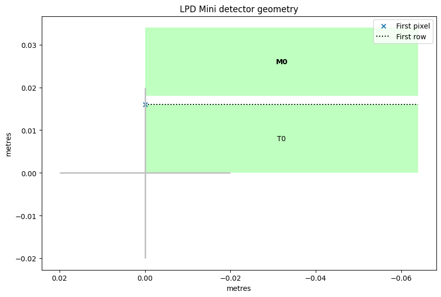
LPD Mini
LPD Mini consists of one or more modules, each with 64×128 pixels, made up of two 32×128 tiles.
The approximate layout of one LPD Mini module, in a front view (looking along the beam).
- class extra_geom.LPD_MiniGeometry(modules, filename='No file', metadata=None)
Detector Layout for LPD Mini.
The coordinates used in this class are 3D (x, y, z), and represent metres.
You won’t normally instantiate this class directly: use one of the constructor class methods to create or load a geometry.
- classmethod from_module_positions(positions, rotations=None, asic_gap=None, unit=0.001)
Generate a geometry for one or more LPD mini modules
Pass a list of (x, y) corner positions. In the default orientation, they refer to the bottom left corner, looking at the module from in front of the sensor.
You can also pass a list of rotations, in degrees. The default (0) orientation has the longer axis (128 pixels) horizontal, with the first tile on the bottom. Each angle rotates the relevant module clockwise, as viewed from in front of the sensor, so an angle of 90 puts the ‘top’ side of the module on the right, seen from the front.
asic_gap specifies the gap between the two tiles in each module. The default is 2mm.
The default units of positions and asic_gap are millimetres. Other units may be used by specifying unit as a length in metres.
- classmethod example(n_modules=1)
Create an example geometry (useful for quick visualization).
- offset(shift, *, modules=slice(None, None, None), tiles=slice(None, None, None))
Move part or all of the detector, making a new geometry.
By default, this moves all modules & tiles. To move the centre down in the image, move the whole geometry up relative to it.
Returns a new geometry object of the same type.
# Move the whole geometry up 2 mm (relative to the beam)
geom2 = geom.offset((0, 2e-3))

# Move quadrant 1 (modules 0, 1, 2, 3) up 2 mm
geom2 = geom.offset((0, 2e-3), modules=np.s_[0:4])

# Move each module by a separate amount
shifts = np.zeros((16, 3))
shifts[5] = (0, 2e-3, 0)    # x, y, z for individual modules
shifts[10] = (0, -1e-3, 0)
geom2 = geom.offset(shifts)
- Parameters:
shift (numpy.ndarray or tuple) – (x, y) or (x, y, z) shift to apply in metres. Can be a single shift for all selected modules, a 2D array with a shift per module, or a 3D array with a shift per tile (
arr[module, tile, xyz]).modules (slice) – Select modules to move; defaults to all modules. Like all Python slicing, the end number is excluded, so
np.s_[:4]moves modules 0, 1, 2, 3.tiles (slice) – Select tiles to move within each module; defaults to all tiles.
- rotate(angles, center=None, modules=slice(None, None, None), tiles=slice(None, None, None), degrees=True)
Rotate part or all of the detector, making a new geometry.
The rotation is defined by composition of rotations about the axes of the coordinate system (https://en.wikipedia.org/wiki/Euler_angles), i.e. a rotation around the z axis rotates the xy (detector) plan. We use the right-hand rule, xy being the detector plan with z increasing looking toward the detector front plan, x increasing to the left, y increasing to the top. Positive rotations are clockwise.
In other words:
Positive x angles tilt the top edge of the detector backwards, away from the source
Positive y angles tilt the right-hand edge (looking along the beam) away from the source
Positive z angles turn the detector clockwise (looking along the beam)
By default, this rotates all modules & tiles. Returns a new geometry object of the same type.
# Rotate the whole geometry by 90 degree in the xy plan
geom2 = geom.rotate((0, 0, 90))

# Move the tile 0 in the module 0 around its center by 90 degrees
geom2 = geom.rotate((0, 0, 90), modules=np.s_[:1], tiles=np.s_[:1])

# Rotate each module by a separate amount
rotate = np.zeros((16, 3))
rotate[5] = (3, 5, 1)  # x, y, z for individual modules
rotate[10] = (0, -2, 1)
geom2 = geom.rotate(rotate)
- Parameters:
angles (np.array or tuple) – (x, y, z) rotations to apply in degree. Can be a single rotation for all selected modules, a 2D array with a rotation per module, or a 3D array with a rotation per tile (
arr[module, tile, xyz]).center (np.array or tuple) – center of rotation. Shape must match angles.shape. If set to None (default), the rotation center is set to: * all modules: center of the detector * selected modules: centers of modules * selected tiles: centers of tiles
modules (slice) – Select modules to rotate; defaults to all modules.
tiles (slice) – Select tiles to move within each module; defaults to all tiles.
degrees (bool) – If True (default), angles are in degrees. If False, angles are in radians.
- write_crystfel_geom(filename, *, data_path=None, mask_path=None, dims=('frame', 'modno', 'ss', 'fs'), nquads=None, adu_per_ev=None, clen=None, photon_energy=None)
Write this geometry to a CrystFEL format (.geom) geometry file.
If the geometry was read from a
.geomfile byfrom_crystfel_geom(), some of the optional fields will be filled from metadata if not specified.- Parameters:
filename (str) – Filename of the geometry file to write.
data_path (str) – Path to the group that contains the data array in the hdf5 file. Default:
'/entry_1/instrument_1/detector_1/data'.mask_path (str) – Path to the group that contains the mask array in the hdf5 file.
dims (tuple) – Dimensions of the data. Extra dimensions, except for the defaults, should be added by their index, e.g. (‘frame’, ‘modno’, 0, ‘ss’, ‘fs’) for raw data. Default:
('frame', 'modno', 'ss', 'fs'). Note: the dimensions must contain frame, ss, fs.adu_per_ev (float) – ADU (analog digital units) per electron volt for the considered detector.
clen (float) – Distance between sample and detector in meters
photon_energy (float) – Beam wave length in eV
- get_pixel_positions(centre=True)
Get the physical coordinates of each pixel in the detector
The output is an array with shape like the data, with an extra dimension of length 3 to hold (x, y, z) coordinates. Coordinates are in metres.
If centre=True, the coordinates are calculated for the centre of each pixel. If not, the coordinates are for the first corner of the pixel (the one nearest the [0, 0] corner of the tile in data space).
- to_distortion_array(allow_negative_xy=False)
Generate a distortion array for pyFAI from this geometry.
- to_pyfai_detector(**kwargs)
Make a PyFAI detector object for JUNGFRAU detector.
You can use PyFAI to azimuthally integrate detector images around the centre point of the geometry. The detector object holds the positions of all the pixels. See the examples for how to use this.
- plot_data(data, *, axis_units='px', frontview=True, ax=None, figsize=None, colorbar=True, interpolate=False, **kwargs)
Plot data from the detector using this geometry.
This approximates or interpolate (with interpolate=True) the geometry to align all pixels to a 2D grid.
Returns a matplotlib axes object.
This method was previously called
plot_data_fast, and can still be called with that name.- Parameters:
data (ndarray) – Should have exactly 3 dimensions, for the modules, then the slow scan and fast scan pixel dimensions.
axis_units (str) – Show the detector scale in pixels (‘px’) or metres (‘m’).
frontview (bool) – If True (the default), x increases to the left, as if you were looking along the beam. False gives a ‘looking into the beam’ view.
ax (~matplotlib.axes.Axes object, optional) – Axes that will be used to draw the image. If None is given (default) a new axes object will be created.
figsize (tuple) – Size of the figure (width, height) in inches to be drawn (default: (10, 10))
colorbar (bool, dict) – Draw colobar with default values (if boolean is given). Colorbar appearance can be controlled by passing a dictionary of properties.
interpolate (bool) – If True, use interpolation when drawing the image.
kwargs – Additional keyword arguments passed to ~matplotlib.imshow
- output_array_for_position(extra_shape=(), dtype=<class 'numpy.float32'>)
Make an empty output array to use with position_modules
You can speed up assembling images by reusing the same output array: call this once, and then pass the array as the
out=parameter toposition_modules(). By default, it allocates a new array on each call, which can be slow.- Parameters:
extra_shape (tuple, optional) – By default, a 2D output array is generated, to assemble a single detector image. If you are assembling multiple pulses at once, pass
extra_shape=(nframes,)to get a 3D output array.dtype (optional (Default: np.float32))
- position_modules_interpolate(data, *, oversample: int = 1, output_pixel_size=None, resize: bool = True, method: str = 'LUT', empty=nan, device: str | None = None, dis_kwargs: dict | None = None)
Assemble data onto a regular grid using pixel-splitting.
This uses pyFAI’s distortion correction machinery to produce an output image corrected from spatial distortion.
- Parameters:
data (ndarray or xarray.DataArray) – Detector data shaped like
expected_data_shape, optionally with extra leading dimensions.oversample (int) – Subdivide output pixels by this factor in each dimension.
output_pixel_size (float or (float, float), optional) – Output pixel size in metres as
(x, y). If omitted, defaults to the detector pixel size.resize (bool) – If True (default), expand the output array to include all pixels so total signal is preserved.
method (str) – pyFAI distortion backend, e.g. “CSR” or “LUT” (default).
empty (float) – Value for empty output pixels.
device (str, optional) – Name of the device: None for OpenMP, “cpu” or “gpu” or the id of the OpenCL device a 2-tuple of integer.
dis_kwargs (dict, optional) – Extra arguments passed to pyFAI’s
Distortion.correct_ng().
- Returns:
out (ndarray) – Assembled image array (counts), with the module dimension removed.
centre (ndarray) – (y, x) output pixel coordinates of the detector centre.
- position_modules_symmetric(data, out=None, threadpool=None)
Assemble data with the centre in the middle of the output array.
The assembly process is the same as
position_modules(), aligning each module to a single pixel grid. But this makes the output array symmetric, with the centre at (height // 2, width // 2).- Parameters:
data (ndarray or xarray.DataArray) – The last three dimensions should match the modules, then the slow scan and fast scan pixel dimensions. If an xarray labelled array is given, it must have a ‘module’ dimension.
out (ndarray, optional) – An output array to assemble the image into. By default, a new array is created at the minimum size to allow symmetric assembly. If an array is passed in, its last two dimensions must be at least this size.
threadpool (concurrent.futures.ThreadPoolExecutor, optional) – If passed, parallelise copying data into the output image. See
position_modules()for details.
- Returns:
out – Array with one dimension fewer than the input. The last two dimensions represent pixel y and x in the detector space.
- Return type:
ndarray
- inspect(axis_units='px', frontview=True)
Plot the 2D layout of this detector geometry.
Returns a matplotlib Axes object.
- compare(other, scale=1.0)
Show a comparison of this geometry with another in a 2D plot.
This shows the current geometry like
inspect(), with the addition of arrows showing how each panel is shifted in the other geometry.- Parameters:
other (DetectorGeometryBase) – A second geometry object to compare with this one. It should be for the same kind of detector.
scale (float) – Scale the arrows showing the difference in positions. This is useful to show small differences clearly.
- data_coords_to_positions(module_no, slow_scan, fast_scan)
Convert data array coordinates to physical positions
Data array coordinates are how you might refer to a pixel in an array of detector data: module number, and indices in the slow-scan and fast-scan directions. But coordinates in the two pixel dimensions aren’t necessarily integers, e.g. if they refer to the centre of a peak.
module_no, fast_scan and slow_scan should all be numpy arrays of the same shape. module_no should hold integers, starting from 0, so 0: Q1M1, 1: Q1M2, etc.
slow_scan and fast_scan describe positions within that module. They may hold floats for sub-pixel positions. In both, 0.5 is the centre of the first pixel.
Returns an array of similar shape with an extra dimension of length 3, for (x, y, z) coordinates in metres.
See also
Converting array coordinates to physical positions demonstrates using this method.
DSSC-1M
DSSC-1M consists of 16 modules of 128×512 pixels each. Each module is further subdivided into 2 sensor tiles, which this geometry code can position independently.
The approximate layout of DSSC-1M, in a front view (looking along the beam).
The pixels in each DSSC module are tesselating hexagons.
This is handled in get_pixel_positions() and
to_distortion_array(), but assembling an image treats
the pixels as rectangles to simplify processing.
This is adequate for previewing detector images, but some pixels will be
approximately half a pixel width from their true position.
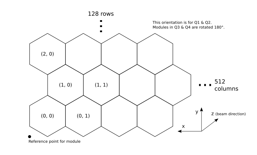
Detail of hexagonal pixels in the corner of one DSSC module.
- class extra_geom.DSSC_1MGeometry(modules, filename='No file', metadata=None)
Detector layout for DSSC-1M
The coordinates used in this class are 3D (x, y, z), and represent metres.
You won’t normally instantiate this class directly: use one of the constructor class methods to create or load a geometry.
- classmethod from_quad_positions(quad_pos, *, unit=0.001, asic_gap=None, panel_gap=None)
Generate a DSSC-1M geometry from quadrant positions.
This produces an idealised geometry, assuming all modules are perfectly flat, aligned and equally spaced within their quadrant.
The position given should refer to the bottom right (looking along the beam) corner of the quadrant.
The origin of the coordinates is in the centre of the detector. Coordinates increase upwards and to the left (looking along the beam).
- Parameters:
quad_pos (list of 2-tuples) – (x, y) coordinates of the last corner (the one by module 4) of each quadrant.
unit (float, optional) – The conversion factor to put the coordinates into metres. The default 1e-3 means the numbers are in millimetres.
asic_gap (float, optional) – The gap between adjacent tiles/ASICs. The default is 2 mm.
panel_gap (float, optional) – The gap between adjacent modules/panels. The default is 4 mm.
- classmethod from_h5_file_and_quad_positions(path, positions, unit=0.001)
Load a DSSC geometry from an XFEL HDF5 format geometry file
The position given should refer to the bottom right (looking along the beam) corner of the quadrant. The passed positions override quadrant positions from the file, if it contains them: see
from_h5_file()to use them.By default, both the quadrant positions and the positions in the file are measured in millimetres; the unit parameter controls this.
The origin of the coordinates is in the centre of the detector. Coordinates increase upwards and to the left (looking along the beam).
This version of the code only handles x and y translation, as this is all that is recorded in the initial LPD geometry file.
- Parameters:
path (str) – Path of an EuXFEL format (HDF5) geometry file for DSSC.
positions (list of 2-tuples) – (x, y) coordinates of the corner of each quadrant (the one with lowest x and y coordinates).
unit (float, optional) – The conversion factor to put the coordinates into metres. The default 1e-3 means the numbers are in millimetres.
- classmethod from_h5_file(path)
Load a DSSC geometry from an XFEL HDF5 format geometry file
This requires a file containing quadrant positions, which not all XFEL geometry files do. Use
from_h5_file_and_quad_positions()to load a file which does not have them.- Parameters:
path (str) – Path of an EuXFEL format (HDF5) geometry file for DSSC.
- classmethod example()
Create an example geometry (useful for quick visualization).
- offset(shift, *, modules=slice(None, None, None), tiles=slice(None, None, None))
Move part or all of the detector, making a new geometry.
By default, this moves all modules & tiles. To move the centre down in the image, move the whole geometry up relative to it.
Returns a new geometry object of the same type.
# Move the whole geometry up 2 mm (relative to the beam)
geom2 = geom.offset((0, 2e-3))

# Move quadrant 1 (modules 0, 1, 2, 3) up 2 mm
geom2 = geom.offset((0, 2e-3), modules=np.s_[0:4])

# Move each module by a separate amount
shifts = np.zeros((16, 3))
shifts[5] = (0, 2e-3, 0)    # x, y, z for individual modules
shifts[10] = (0, -1e-3, 0)
geom2 = geom.offset(shifts)
- Parameters:
shift (numpy.ndarray or tuple) – (x, y) or (x, y, z) shift to apply in metres. Can be a single shift for all selected modules, a 2D array with a shift per module, or a 3D array with a shift per tile (
arr[module, tile, xyz]).modules (slice) – Select modules to move; defaults to all modules. Like all Python slicing, the end number is excluded, so
np.s_[:4]moves modules 0, 1, 2, 3.tiles (slice) – Select tiles to move within each module; defaults to all tiles.
- rotate(angles, center=None, modules=slice(None, None, None), tiles=slice(None, None, None), degrees=True)
Rotate part or all of the detector, making a new geometry.
The rotation is defined by composition of rotations about the axes of the coordinate system (https://en.wikipedia.org/wiki/Euler_angles), i.e. a rotation around the z axis rotates the xy (detector) plan. We use the right-hand rule, xy being the detector plan with z increasing looking toward the detector front plan, x increasing to the left, y increasing to the top. Positive rotations are clockwise.
In other words:
Positive x angles tilt the top edge of the detector backwards, away from the source
Positive y angles tilt the right-hand edge (looking along the beam) away from the source
Positive z angles turn the detector clockwise (looking along the beam)
By default, this rotates all modules & tiles. Returns a new geometry object of the same type.
# Rotate the whole geometry by 90 degree in the xy plan
geom2 = geom.rotate((0, 0, 90))

# Move the tile 0 in the module 0 around its center by 90 degrees
geom2 = geom.rotate((0, 0, 90), modules=np.s_[:1], tiles=np.s_[:1])

# Rotate each module by a separate amount
rotate = np.zeros((16, 3))
rotate[5] = (3, 5, 1)  # x, y, z for individual modules
rotate[10] = (0, -2, 1)
geom2 = geom.rotate(rotate)
- Parameters:
angles (np.array or tuple) – (x, y, z) rotations to apply in degree. Can be a single rotation for all selected modules, a 2D array with a rotation per module, or a 3D array with a rotation per tile (
arr[module, tile, xyz]).center (np.array or tuple) – center of rotation. Shape must match angles.shape. If set to None (default), the rotation center is set to: * all modules: center of the detector * selected modules: centers of modules * selected tiles: centers of tiles
modules (slice) – Select modules to rotate; defaults to all modules.
tiles (slice) – Select tiles to move within each module; defaults to all tiles.
degrees (bool) – If True (default), angles are in degrees. If False, angles are in radians.
- quad_positions(h5_file=None)
Get the positions of the 4 quadrants
Quadrant positions are returned as (x, y) coordinates in millimetres. Their meaning is as in
from_h5_file_and_quad_positions().To use the returned positions with an existing XFEL HDF5 geometry file, the path to that file should be passed in. In that case, the offsets of M1 T1 in each quadrant are read from the file to calculate a suitable quadrant position. The geometry in the file is not checked against this geometry object at all.
- to_h5_file_and_quad_positions(path)
Write this geometry to an XFEL HDF5 format geometry file
The quadrant positions are stored in the file, but also returned. These and the numbers in the file are in millimetres.
The file and quadrant positions produced by this method are compatible with
from_h5_file_and_quad_positions().
- get_pixel_positions(centre=True)
Get the physical coordinates of each pixel in the detector
The output is an array with shape like the data, with an extra dimension of length 3 to hold (x, y, z) coordinates. Coordinates are in metres.
If centre=True, the coordinates are calculated for the centre of each pixel. If not, the coordinates are for the first corner of the pixel (the one nearest the [0, 0] corner of the tile in data space).
- to_distortion_array(allow_negative_xy=False)
Return distortion matrix for DSSC detector, suitable for pyFAI.
- Parameters:
allow_negative_xy (bool) – If False (default), shift the origin so no x or y coordinates are negative. If True, the origin is the detector centre.
- Returns:
out – Array of float 32 with shape (2048, 512, 6, 3). The dimensions mean:
2048 = 16 modules * 128 pixels (slow scan axis)
512 pixels (fast scan axis)
6 corners of each pixel
3 numbers for z, y, x
- Return type:
ndarray
- to_pyfai_detector(**kwargs)
Make a PyFAI detector object for this detector
You can use PyFAI to azimuthally integrate detector images around the centre point of the geometry. The detector object holds the positions of all the pixels. See the examples for how to use this.
- plot_data(data, *, axis_units='px', frontview=True, ax=None, figsize=None, colorbar=False, **kwargs)
Plot data from the detector using this geometry.
This approximates or interpolate (with interpolate=True) the geometry to align all pixels to a 2D grid.
Returns a matplotlib axes object.
This method was previously called
plot_data_fast, and can still be called with that name.- Parameters:
data (ndarray) – Should have exactly 3 dimensions, for the modules, then the slow scan and fast scan pixel dimensions.
axis_units (str) – Show the detector scale in pixels (‘px’) or metres (‘m’).
frontview (bool) – If True (the default), x increases to the left, as if you were looking along the beam. False gives a ‘looking into the beam’ view.
ax (~matplotlib.axes.Axes object, optional) – Axes that will be used to draw the image. If None is given (default) a new axes object will be created.
figsize (tuple) – Size of the figure (width, height) in inches to be drawn (default: (10, 10))
colorbar (bool, dict) – Draw colobar with default values (if boolean is given). Colorbar appearance can be controlled by passing a dictionary of properties.
interpolate (bool) – If True, use interpolation when drawing the image.
kwargs – Additional keyword arguments passed to ~matplotlib.imshow
- plot_data_cartesian(data, **kwargs)
Plot the given data converted to square pixels
This converts the data from DSSC’s hexagonal pixels to a similar number of pixels on a square grid, and displays the image. It accepts all the same keyword arguments as
plot_data().
- plot_data_hexes(data, *, frontview=True, ax=None, figsize=None, colorbar=False, vmin=None, vmax=None, norm=None, cmap=None, module=None)
Plot data from the detector showing hexagonal pixels
Most of the arguments are like those for
plot_data(). This method is slower, but sometimes useful to look at small details. It can also plot data for a single module, if you pass a suitable 2D array as data and a module number as module.
- position_modules(data, out=None, threadpool=None)
Assemble data from this detector according to where the pixels are.
This approximates the geometry to align all pixels to a 2D grid.
This method was previously called
position_modules_fast, and can still be called with that name.- Parameters:
data (ndarray or xarray.DataArray) – The last three dimensions should match the modules, then the slow scan and fast scan pixel dimensions. If an xarray labelled array is given, it must have a ‘module’ dimension.
out (ndarray, optional) – An output array to assemble the image into. By default, a new array is allocated. Use
output_array_for_position()to create a suitable array. If an array is passed in, it must match the dtype of the data and the shape of the array that would have been allocated. Parts of the array not covered by detector tiles are not overwritten. In general, you can reuse an output array if you are assembling similar pulses or pulse trains with the same geometry.threadpool (concurrent.futures.ThreadPoolExecutor, optional) – If passed, parallelise copying data into the output image. By default, data for different tiles are copied serially. For a single 1 MPx image, the default appears to be faster, but for assembling a stack of several images at once, multithreading can help.
- Returns:
out (ndarray) – Array with one dimension fewer than the input. The last two dimensions represent pixel y and x in the detector space.
centre (ndarray) – (y, x) pixel location of the detector centre in this geometry.
- position_modules_cartesian(data, out=None, threadpool=None)
Assemble DSSC data on a square pixel grid
This converts the data from DSSC’s hexagonal pixels to a similar number of pixels on a square grid, and displays the image. The arguments are the same as for
position_modules().
- output_array_for_position(extra_shape=(), dtype=<class 'numpy.float32'>)
Make an empty output array to use with position_modules
You can speed up assembling images by reusing the same output array: call this once, and then pass the array as the
out=parameter toposition_modules(). By default, it allocates a new array on each call, which can be slow.- Parameters:
extra_shape (tuple, optional) – By default, a 2D output array is generated, to assemble a single detector image. If you are assembling multiple pulses at once, pass
extra_shape=(nframes,)to get a 3D output array.dtype (optional (Default: np.float32))
- inspect(axis_units='px', frontview=True)
Plot the 2D layout of this detector geometry.
Returns a matplotlib Axes object.
- compare(other, scale=1.0)
Show a comparison of this geometry with another in a 2D plot.
This shows the current geometry like
inspect(), with the addition of arrows showing how each panel is shifted in the other geometry.- Parameters:
other (DetectorGeometryBase) – A second geometry object to compare with this one. It should be for the same kind of detector.
scale (float) – Scale the arrows showing the difference in positions. This is useful to show small differences clearly.
JUNGFRAU
JUNGFRAU detectors can be made with varying numbers of 512×1024 pixel modules. Each module is further subdivided into 8 sensor tiles.
Note
Reading & writing geometry files for JUNGFRAU is not yet implemented.
- class extra_geom.JUNGFRAUGeometry(modules, filename='No file', metadata=None)
Detector layout for flexible Jungfrau arrangements
The base JUNGFRAU unit (and rigid group) in combined arrangements is the JF-500K module, which is an independent detector unit of 2 x 4 ASIC tiles.
In the default orientation, the slow-scan dimension is y and the fast-scan dimension is x, so the data shape for one module is (y, x).
- classmethod from_module_positions(offsets=((0, 0),), orientations=None, asic_gap=2, unit=7.5e-05)
Generate a Jungfrau geometry object from module positions
- Parameters:
offsets (iterable of tuples) –
iterable of length n_modules containing a coordinate tuple (x,y) for each offset to the global origin. Coordinates are in pixel units by default.
These offsets are positions for the bottom, beam-right corner of each module, regardless of its orientation.
orientations (iterable of tuples) –
list of length n_modules containing a unit-vector tuple (x,y) for each orientation wrt. the axes
Orientations default to (1,1) for each module if this optional keyword argument is lacking; if not, the number of elements must match the number of modules as per offsets
asic_gap (float) – The gap between the 8 ASICs within each module. This is in pixel units by default.
unit (float) – The unit for offsets and asic_gap, in metres. Defaults to the pixel size (75 um).
- classmethod from_crystfel_geom(filename)
Read a CrystFEL format (.geom) geometry file.
Returns a new geometry object.
- classmethod example(n_modules=1)
Create an example geometry (useful for quick visualization).
- write_crystfel_geom(filename, *, data_path=None, mask_path=None, dims=('frame', 'modno', 'ss', 'fs'), nquads=None, adu_per_ev=None, clen=None, photon_energy=None)
Write this geometry to a CrystFEL format (.geom) geometry file.
If the geometry was read from a
.geomfile byfrom_crystfel_geom(), some of the optional fields will be filled from metadata if not specified.- Parameters:
filename (str) – Filename of the geometry file to write.
data_path (str) – Path to the group that contains the data array in the hdf5 file. Default:
'/entry_1/instrument_1/detector_1/data'.mask_path (str) – Path to the group that contains the mask array in the hdf5 file.
dims (tuple) – Dimensions of the data. Extra dimensions, except for the defaults, should be added by their index, e.g. (‘frame’, ‘modno’, 0, ‘ss’, ‘fs’) for raw data. Default:
('frame', 'modno', 'ss', 'fs'). Note: the dimensions must contain frame, ss, fs.adu_per_ev (float) – ADU (analog digital units) per electron volt for the considered detector.
clen (float) – Distance between sample and detector in meters
photon_energy (float) – Beam wave length in eV
- get_pixel_positions(centre=True)
Get the physical coordinates of each pixel in the detector
The output is an array with shape like the data, with an extra dimension of length 3 to hold (x, y, z) coordinates. Coordinates are in metres.
If centre=True, the coordinates are calculated for the centre of each pixel. If not, the coordinates are for the first corner of the pixel (the one nearest the [0, 0] corner of the tile in data space).
- to_distortion_array(allow_negative_xy=False)
Generate a distortion array for pyFAI from this geometry.
- to_pyfai_detector(**kwargs)
Make a PyFAI detector object for JUNGFRAU detector.
You can use PyFAI to azimuthally integrate detector images around the centre point of the geometry. The detector object holds the positions of all the pixels. See the examples for how to use this.
- plot_data(data, *, axis_units='px', frontview=True, ax=None, figsize=None, colorbar=True, **kwargs)
Plot data from the detector using this geometry.
This approximates or interpolate (with interpolate=True) the geometry to align all pixels to a 2D grid.
Returns a matplotlib axes object.
This method was previously called
plot_data_fast, and can still be called with that name.- Parameters:
data (ndarray) – Should have exactly 3 dimensions, for the modules, then the slow scan and fast scan pixel dimensions.
axis_units (str) – Show the detector scale in pixels (‘px’) or metres (‘m’).
frontview (bool) – If True (the default), x increases to the left, as if you were looking along the beam. False gives a ‘looking into the beam’ view.
ax (~matplotlib.axes.Axes object, optional) – Axes that will be used to draw the image. If None is given (default) a new axes object will be created.
figsize (tuple) – Size of the figure (width, height) in inches to be drawn (default: (10, 10))
colorbar (bool, dict) – Draw colobar with default values (if boolean is given). Colorbar appearance can be controlled by passing a dictionary of properties.
interpolate (bool) – If True, use interpolation when drawing the image.
kwargs – Additional keyword arguments passed to ~matplotlib.imshow
- position_modules_interpolate(data, **kwargs)
Assemble data onto a regular grid using pixel-splitting.
This uses pyFAI’s distortion correction machinery to produce an output image corrected from spatial distortion.
- Parameters:
data (ndarray or xarray.DataArray) – Detector data shaped like
expected_data_shape, optionally with extra leading dimensions.oversample (int) – Subdivide output pixels by this factor in each dimension.
output_pixel_size (float or (float, float), optional) – Output pixel size in metres as
(x, y). If omitted, defaults to the detector pixel size.resize (bool) – If True (default), expand the output array to include all pixels so total signal is preserved.
method (str) – pyFAI distortion backend, e.g. “CSR” or “LUT” (default).
empty (float) – Value for empty output pixels.
device (str, optional) – Name of the device: None for OpenMP, “cpu” or “gpu” or the id of the OpenCL device a 2-tuple of integer.
dis_kwargs (dict, optional) – Extra arguments passed to pyFAI’s
Distortion.correct_ng().
- Returns:
out (ndarray) – Assembled image array (counts), with the module dimension removed.
centre (ndarray) – (y, x) output pixel coordinates of the detector centre.
- position_modules(data, out=None, threadpool=None)
Assemble data from this detector according to where the pixels are.
This approximates the geometry to align all pixels to a 2D grid.
This method was previously called
position_modules_fast, and can still be called with that name.- Parameters:
data (ndarray or xarray.DataArray) – The last three dimensions should match the modules, then the slow scan and fast scan pixel dimensions. If an xarray labelled array is given, it must have a ‘module’ dimension.
out (ndarray, optional) – An output array to assemble the image into. By default, a new array is allocated. Use
output_array_for_position()to create a suitable array. If an array is passed in, it must match the dtype of the data and the shape of the array that would have been allocated. Parts of the array not covered by detector tiles are not overwritten. In general, you can reuse an output array if you are assembling similar pulses or pulse trains with the same geometry.threadpool (concurrent.futures.ThreadPoolExecutor, optional) – If passed, parallelise copying data into the output image. By default, data for different tiles are copied serially. For a single 1 MPx image, the default appears to be faster, but for assembling a stack of several images at once, multithreading can help.
- Returns:
out (ndarray) – Array with one dimension fewer than the input. The last two dimensions represent pixel y and x in the detector space.
centre (ndarray) – (y, x) pixel location of the detector centre in this geometry.
- output_array_for_position(extra_shape=(), dtype=<class 'numpy.float32'>)
Make an empty output array to use with position_modules
You can speed up assembling images by reusing the same output array: call this once, and then pass the array as the
out=parameter toposition_modules(). By default, it allocates a new array on each call, which can be slow.- Parameters:
extra_shape (tuple, optional) – By default, a 2D output array is generated, to assemble a single detector image. If you are assembling multiple pulses at once, pass
extra_shape=(nframes,)to get a 3D output array.dtype (optional (Default: np.float32))
- inspect(axis_units='px', frontview=True, module_names=[])
Plot the 2D layout of this detector geometry.
Returns a matplotlib Axes object.
- compare(other, scale=1.0)
Show a comparison of this geometry with another in a 2D plot.
This shows the current geometry like
inspect(), with the addition of arrows showing how each panel is shifted in the other geometry.- Parameters:
other (DetectorGeometryBase) – A second geometry object to compare with this one. It should be for the same kind of detector.
scale (float) – Scale the arrows showing the difference in positions. This is useful to show small differences clearly.
- data_coords_to_positions(module_no, slow_scan, fast_scan)
Convert data array coordinates to physical positions
Data array coordinates are how you might refer to a pixel in an array of detector data: module number, and indices in the slow-scan and fast-scan directions. But coordinates in the two pixel dimensions aren’t necessarily integers, e.g. if they refer to the centre of a peak.
module_no, fast_scan and slow_scan should all be numpy arrays of the same shape. module_no should hold integers, starting from 0, so 0: Q1M1, 1: Q1M2, etc.
slow_scan and fast_scan describe positions within that module. They may hold floats for sub-pixel positions. In both, 0.5 is the centre of the first pixel.
Returns an array of similar shape with an extra dimension of length 3, for (x, y, z) coordinates in metres.
See also
Converting array coordinates to physical positions demonstrates using this method.
PNCCD
PNCCD detectors have two movable modules of 1024×512 pixels, each of which is a single tile.
- class extra_geom.PNCCDGeometry(modules, filename='No file', metadata=None)
Detector layout for pnCCD
The large-area, pn-junction Charge Coupled Device detector consists of two movable modules with a single tile each.
In its default configuration, the complete detector frame is read out and written to file as a single image, with the modules split along the slow-scan dimension y. The public methods of this type support both the combined image array as well as separated module with
expected_data_shape.- expected_data_shape = (2, 512, 1024)
- classmethod from_relative_positions(gap=0.004, top_offset=(0.0, 0.0, 0.0), bottom_offset=(0.0, 0.0, 0.0))
Generate a pnCCD geometry from relative module positions.
The modules are assumed to be separated by the a gap centered around the beam (at the origin) in x, y and z = 0, with an optional offset applied to each module.
- Parameters:
gap (float) – The gap between the detector modules centered around the beam, 4mm (~50 px) by default.
top_offset (array_like of length 3) – Optional offset (x, y, z) for each module relative to the centered position.
bottom_offset (array_like of length 3) – Optional offset (x, y, z) for each module relative to the centered position.
- classmethod from_absolute_positions(top, bottom)
Generate a pnCCD geometry from absolute module positions.
- Parameters:
top (array_like of length 3) – Absolute position (x, y, z) for the first pixel of each module.
bottom (array_like of length 3) – Absolute position (x, y, z) for the first pixel of each module.
- classmethod example()
Create an example geometry (useful for quick visualization).
- plot_data(data, *args, **kwargs)
Plot data from the detector using this geometry.
This approximates or interpolate (with interpolate=True) the geometry to align all pixels to a 2D grid.
Returns a matplotlib axes object.
This method was previously called
plot_data_fast, and can still be called with that name.- Parameters:
data (ndarray) – Should have exactly 3 dimensions, for the modules, then the slow scan and fast scan pixel dimensions.
axis_units (str) – Show the detector scale in pixels (‘px’) or metres (‘m’).
frontview (bool) – If True (the default), x increases to the left, as if you were looking along the beam. False gives a ‘looking into the beam’ view.
ax (~matplotlib.axes.Axes object, optional) – Axes that will be used to draw the image. If None is given (default) a new axes object will be created.
figsize (tuple) – Size of the figure (width, height) in inches to be drawn (default: (10, 10))
colorbar (bool, dict) – Draw colobar with default values (if boolean is given). Colorbar appearance can be controlled by passing a dictionary of properties.
interpolate (bool) – If True, use interpolation when drawing the image.
kwargs – Additional keyword arguments passed to ~matplotlib.imshow
- position_modules_interpolate(data, *args, **kwargs)
Assemble data onto a regular grid using pixel-splitting.
This uses pyFAI’s distortion correction machinery to produce an output image corrected from spatial distortion.
- Parameters:
data (ndarray or xarray.DataArray) – Detector data shaped like
expected_data_shape, optionally with extra leading dimensions.oversample (int) – Subdivide output pixels by this factor in each dimension.
output_pixel_size (float or (float, float), optional) – Output pixel size in metres as
(x, y). If omitted, defaults to the detector pixel size.resize (bool) – If True (default), expand the output array to include all pixels so total signal is preserved.
method (str) – pyFAI distortion backend, e.g. “CSR” or “LUT” (default).
empty (float) – Value for empty output pixels.
device (str, optional) – Name of the device: None for OpenMP, “cpu” or “gpu” or the id of the OpenCL device a 2-tuple of integer.
dis_kwargs (dict, optional) – Extra arguments passed to pyFAI’s
Distortion.correct_ng().
- Returns:
out (ndarray) – Assembled image array (counts), with the module dimension removed.
centre (ndarray) – (y, x) output pixel coordinates of the detector centre.
- position_modules(data, *args, **kwargs)
Assemble data from this detector according to where the pixels are.
This approximates the geometry to align all pixels to a 2D grid.
This method was previously called
position_modules_fast, and can still be called with that name.- Parameters:
data (ndarray or xarray.DataArray) – The last three dimensions should match the modules, then the slow scan and fast scan pixel dimensions. If an xarray labelled array is given, it must have a ‘module’ dimension.
out (ndarray, optional) – An output array to assemble the image into. By default, a new array is allocated. Use
output_array_for_position()to create a suitable array. If an array is passed in, it must match the dtype of the data and the shape of the array that would have been allocated. Parts of the array not covered by detector tiles are not overwritten. In general, you can reuse an output array if you are assembling similar pulses or pulse trains with the same geometry.threadpool (concurrent.futures.ThreadPoolExecutor, optional) – If passed, parallelise copying data into the output image. By default, data for different tiles are copied serially. For a single 1 MPx image, the default appears to be faster, but for assembling a stack of several images at once, multithreading can help.
- Returns:
out (ndarray) – Array with one dimension fewer than the input. The last two dimensions represent pixel y and x in the detector space.
centre (ndarray) – (y, x) pixel location of the detector centre in this geometry.
- output_array_for_position(extra_shape=(), dtype=<class 'numpy.float32'>)
Make an empty output array to use with position_modules
You can speed up assembling images by reusing the same output array: call this once, and then pass the array as the
out=parameter toposition_modules(). By default, it allocates a new array on each call, which can be slow.- Parameters:
extra_shape (tuple, optional) – By default, a 2D output array is generated, to assemble a single detector image. If you are assembling multiple pulses at once, pass
extra_shape=(nframes,)to get a 3D output array.dtype (optional (Default: np.float32))
- inspect(axis_units='px', frontview=True)
Plot the 2D layout of this detector geometry.
Returns a matplotlib Figure object.
- compare(other, scale=1.0)
Show a comparison of this geometry with another in a 2D plot.
This shows the current geometry like
inspect(), with the addition of arrows showing how each panel is shifted in the other geometry.- Parameters:
other (DetectorGeometryBase) – A second geometry object to compare with this one. It should be for the same kind of detector.
scale (float) – Scale the arrows showing the difference in positions. This is useful to show small differences clearly.
ePix100/ePix10K
ePix100 detectors have one module of 704 × 768 pixels. Module built from 4 ASICs with 352 rows and 384 columns of pixels with wide pixes on inner edges. Normal pixels are 50 × 50 um.
ePix10K detectors have one module of 352 × 384 pixels. Module built from 4 ASICs with 176 rows and 192 columns of pixels with wide pixes on inner edges. Normal pixels are 100 × 100 um.
Note
Only methods unique to the Epix100Geometry class are
documented, but it otherwise has the same interface as
Epix10KGeometry.
- class extra_geom.Epix100Geometry(modules, filename='No file', metadata=None)
Detector layout for ePix100
ePix100 detectors have one module, which is built from 4 ASICs with wide pixes on inner edges.
In its default configuration, the complete detector frame is read out and written to file as a single image, with the ASICs split along the both dimensions.
There are 4 more rows in raw data. These are calibration pixels. They have the same electronics as normal pixels but aren’t wired to the sensor. They are two first and two last rows in the raw data array. This class assumes that calibration rows are cut.
Note
The ePix100 has 2 different geometry layouts:
A single monolithic sensor with a 2x2 array of four ASICs bonded to it. These would have no dead gaps but would have large pixels in the central cross. Use
Epix10KGeometry.monolithic_geometry()to generate this geometry.A pair of sensors with each sensor being bonded to two ASICs. These would have a dead gap equal to twice the guard ring width (~450-500um) plus a mechanical gap of about 200-300 microns. This would result in a total dead gap of about 1.25 millimeters. For this case use
pair_geometry().
- classmethod from_relative_positions(asic_gap=None, unit=None, top=(0.0, 0.0, 0.0), bottom=(0.0, 0.0, 0.0))
Generate an ePix100 geometry from relative ASICS-pair positions.
- Parameters:
asic_gap (float) – The gap between asics within a pair (default 250um)
unit (float) – To give positions in units other than pixels, pass the unit parameter as the length of the unit in metres. E.g.
unit=1e-3means the coordinates are in millimetres.top (array_like of length 3 Optional) – offset (x, y, z) for asic pair relative to the centered position.
bottom (array_like of length 3 Optional) – offset (x, y, z) for asic pair relative to the centered position.
- classmethod pair_geometry()
Return the geometry for an ePix100 with a pair of sensors.
One can determine the exact gap existing between the 2 (top and bottom) ASIC pairs. A rough estimation of the gap has been seen at ~25 pixels, which is what this method will generate a geometry with.
- class extra_geom.Epix10KGeometry(modules, filename='No file', metadata=None)
Detector layout for ePix10K
ePix10K detectors have one module, which is built from 4 ASICs with wide pixes on inner edges.
In its default configuration, the complete detector frame is read out and written to file as a single image, with the ASICs split along the both dimensions.
There are 4 more rows in raw data. These are calibration pixels. They have the same electronics as normal pixels but aren’t wired to the sensor. They are two first and two last rows in the raw data array. This class assumes that calibration rows are cut.
- classmethod from_origin(origin=(0, 0), asic_gap=None, unit=None)
Generate a geometry from origin position.
This produces an idealised geometry, assuming all modules are perfectly flat, aligned and equally spaced within the detector.
The default origin (0, 0) of the coordinates is the center of the detector. If another coordinate is given as the origin, it is relative to the center. Coordinates increase upwards and to the left (looking along the beam).
To give positions in units other than pixels, pass the unit parameter as the length of the unit in metres. E.g.
unit=1e-3means the coordinates are in millimetres.
- classmethod from_crystfel_geom(filename)
Read a CrystFEL format (.geom) geometry file.
Returns a new geometry object.
- classmethod monolithic_geometry()
Return the geometry for an ePix100/ePix10K with a single monolithic sensor.
- classmethod example()
Create an example geometry (useful for quick visualization).
- write_crystfel_geom(filename, *, data_path=None, mask_path=None, dims=('frame', 'modno', 'ss', 'fs'), nquads=None, adu_per_ev=None, clen=None, photon_energy=None)
Write this geometry to a CrystFEL format (.geom) geometry file.
If the geometry was read from a
.geomfile byfrom_crystfel_geom(), some of the optional fields will be filled from metadata if not specified.- Parameters:
filename (str) – Filename of the geometry file to write.
data_path (str) – Path to the group that contains the data array in the hdf5 file. Default:
'/entry_1/instrument_1/detector_1/data'.mask_path (str) – Path to the group that contains the mask array in the hdf5 file.
dims (tuple) – Dimensions of the data. Extra dimensions, except for the defaults, should be added by their index, e.g. (‘frame’, ‘modno’, 0, ‘ss’, ‘fs’) for raw data. Default:
('frame', 'modno', 'ss', 'fs'). Note: the dimensions must contain frame, ss, fs.adu_per_ev (float) – ADU (analog digital units) per electron volt for the considered detector.
clen (float) – Distance between sample and detector in meters
photon_energy (float) – Beam wave length in eV
- get_pixel_positions(centre=True)
Get the physical coordinates of each pixel in the detector
The output is an array with shape like the data, with an extra dimension of length 3 to hold (x, y, z) coordinates. Coordinates are in metres.
If centre=True, the coordinates are calculated for the centre of each pixel. If not, the coordinates are for the first corner of the pixel (the one nearest the [0, 0] corner of the tile in data space).
- plot_data(data, *args, **kwargs)
Plot data from the detector using this geometry.
This approximates or interpolate (with interpolate=True) the geometry to align all pixels to a 2D grid.
Returns a matplotlib axes object.
This method was previously called
plot_data_fast, and can still be called with that name.- Parameters:
data (ndarray) – Should have exactly 3 dimensions, for the modules, then the slow scan and fast scan pixel dimensions.
axis_units (str) – Show the detector scale in pixels (‘px’) or metres (‘m’).
frontview (bool) – If True (the default), x increases to the left, as if you were looking along the beam. False gives a ‘looking into the beam’ view.
ax (~matplotlib.axes.Axes object, optional) – Axes that will be used to draw the image. If None is given (default) a new axes object will be created.
figsize (tuple) – Size of the figure (width, height) in inches to be drawn (default: (10, 10))
colorbar (bool, dict) – Draw colobar with default values (if boolean is given). Colorbar appearance can be controlled by passing a dictionary of properties.
interpolate (bool) – If True, use interpolation when drawing the image.
kwargs – Additional keyword arguments passed to ~matplotlib.imshow
- position_modules_interpolate(data, *args, **kwargs)
Assemble data onto a regular grid using pixel-splitting.
This uses pyFAI’s distortion correction machinery to produce an output image corrected from spatial distortion.
- Parameters:
data (ndarray or xarray.DataArray) – Detector data shaped like
expected_data_shape, optionally with extra leading dimensions.oversample (int) – Subdivide output pixels by this factor in each dimension.
output_pixel_size (float or (float, float), optional) – Output pixel size in metres as
(x, y). If omitted, defaults to the detector pixel size.resize (bool) – If True (default), expand the output array to include all pixels so total signal is preserved.
method (str) – pyFAI distortion backend, e.g. “CSR” or “LUT” (default).
empty (float) – Value for empty output pixels.
device (str, optional) – Name of the device: None for OpenMP, “cpu” or “gpu” or the id of the OpenCL device a 2-tuple of integer.
dis_kwargs (dict, optional) – Extra arguments passed to pyFAI’s
Distortion.correct_ng().
- Returns:
out (ndarray) – Assembled image array (counts), with the module dimension removed.
centre (ndarray) – (y, x) output pixel coordinates of the detector centre.
- position_modules(data, *args, **kwargs)
Assemble data from this detector according to where the pixels are.
This approximates the geometry to align all pixels to a 2D grid.
This method was previously called
position_modules_fast, and can still be called with that name.- Parameters:
data (ndarray or xarray.DataArray) – The last three dimensions should match the modules, then the slow scan and fast scan pixel dimensions. If an xarray labelled array is given, it must have a ‘module’ dimension.
out (ndarray, optional) – An output array to assemble the image into. By default, a new array is allocated. Use
output_array_for_position()to create a suitable array. If an array is passed in, it must match the dtype of the data and the shape of the array that would have been allocated. Parts of the array not covered by detector tiles are not overwritten. In general, you can reuse an output array if you are assembling similar pulses or pulse trains with the same geometry.threadpool (concurrent.futures.ThreadPoolExecutor, optional) – If passed, parallelise copying data into the output image. By default, data for different tiles are copied serially. For a single 1 MPx image, the default appears to be faster, but for assembling a stack of several images at once, multithreading can help.
- Returns:
out (ndarray) – Array with one dimension fewer than the input. The last two dimensions represent pixel y and x in the detector space.
centre (ndarray) – (y, x) pixel location of the detector centre in this geometry.
- classmethod normalize_data(data)
Remove diagnostic pixels from the data
EuXFEL ePix data can contain extra rows with diagnostic information. this method remove these row if they are present.
- output_array_for_position(extra_shape=(), dtype=<class 'numpy.float32'>)
Make an empty output array to use with position_modules
You can speed up assembling images by reusing the same output array: call this once, and then pass the array as the
out=parameter toposition_modules(). By default, it allocates a new array on each call, which can be slow.- Parameters:
extra_shape (tuple, optional) – By default, a 2D output array is generated, to assemble a single detector image. If you are assembling multiple pulses at once, pass
extra_shape=(nframes,)to get a 3D output array.dtype (optional (Default: np.float32))
- inspect(axis_units='px', frontview=True)
Plot the 2D layout of this detector geometry.
Returns a matplotlib Axes object.
- compare(other, scale=1.0)
Show a comparison of this geometry with another in a 2D plot.
This shows the current geometry like
inspect(), with the addition of arrows showing how each panel is shifted in the other geometry.- Parameters:
other (DetectorGeometryBase) – A second geometry object to compare with this one. It should be for the same kind of detector.
scale (float) – Scale the arrows showing the difference in positions. This is useful to show small differences clearly.
- classmethod asic_seams()
Make a boolean array marking the wide pixels
This returns a full frame array with False for normal pixels, and True for the wide pixels at inner edges of ASICs.
- classmethod pixel_areas()
Make an array of pixel areas
This returns a full frame array with pixel areas. Pixels on inner edges of ASICs are bigger.
Generic Detector
Generic detector may represent an unconstrained detector of your choice.
- class extra_geom.GenericGeometry(modules, filename='No file', metadata=None)
A generic detector layout based either on the CrystFEL geom file or on a set of parameters.
The coordinates used in this class are 3D (x, y, z), and represent metres.
The
expected_data_shapeis a following triple :the number of modules which is the length of the
corner_coordinatesarraythe number of tiles in a module along the slow-scan direction multiplied by the number of slow-scan pixels per tile
frag_ss_pixelsthe number of tiles in a module along the fast-scan direction multiplied by the number of fast-scan pixels per tile
frag_fs_pixels
- classmethod from_simple_description(pixel_size: float, slow_pixels: int, fast_pixels: int, corner_coordinates: List[ndarray] = [array([0., 0., 0.])], ss_vec: ndarray = array([1, 0, 0]), fs_vec: ndarray = array([0, 1, 0]), n_tiles_per_module: int = 1, tile_gap: float | None = None, tile_vec: ndarray | None = None)
Creates a generic detector from a dictionary.
- Parameters:
pixel_size (float) – the size of a pixel in meters (reversed CrystFEL’s res)
slow_pixels (int) – the size of a tile along the slow- and the fast-scan axes
fast_pixels (int) – the size of a tile along the slow- and the fast-scan axes
corner_coordinates (ndarray) – 3D coordinates of the first pixel of each module
ss_vec (ndarray) – 3D unit vectors of the slow- and the fast-scan directions in the lab coordinates (the X-axis points to the left looking along the beam, the Y-axis points up, and the Z-axis goes with the beam). Example: np.array([0, 1, 0])
fs_vec (ndarray) – 3D unit vectors of the slow- and the fast-scan directions in the lab coordinates (the X-axis points to the left looking along the beam, the Y-axis points up, and the Z-axis goes with the beam). Example: np.array([0, 1, 0])
n_tiles_per_module (int) – the number of tiles in each module, default=1
tile_gap (float) – the gap between two tiles in metres, default=pixel_size
tile_vec (ndarray) – the direction of tile replication, default=[1, 0, 0]
- write_crystfel_geom(filename, *, data_path=None, mask_path=None, dims=('frame', 'modno', 'ss', 'fs'), nquads=None, adu_per_ev=None, clen=None, photon_energy=None)
Write this geometry to a CrystFEL format (.geom) geometry file.
If the geometry was read from a
.geomfile byfrom_crystfel_geom(), some of the optional fields will be filled from metadata if not specified.- Parameters:
filename (str) – Filename of the geometry file to write.
data_path (str) – Path to the group that contains the data array in the hdf5 file. Default:
'/entry_1/instrument_1/detector_1/data'.mask_path (str) – Path to the group that contains the mask array in the hdf5 file.
dims (tuple) – Dimensions of the data. Extra dimensions, except for the defaults, should be added by their index, e.g. (‘frame’, ‘modno’, 0, ‘ss’, ‘fs’) for raw data. Default:
('frame', 'modno', 'ss', 'fs'). Note: the dimensions must contain frame, ss, fs.adu_per_ev (float) – ADU (analog digital units) per electron volt for the considered detector.
clen (float) – Distance between sample and detector in meters
photon_energy (float) – Beam wave length in eV
- get_pixel_positions(centre=True)
Get the physical coordinates of each pixel in the detector
The output is an array with shape like the data, with an extra dimension of length 3 to hold (x, y, z) coordinates. Coordinates are in metres.
If centre=True, the coordinates are calculated for the centre of each pixel. If not, the coordinates are for the first corner of the pixel (the one nearest the [0, 0] corner of the tile in data space).
- plot_data(data, *, axis_units='px', frontview=True, ax=None, figsize=None, colorbar=True, interpolate=False, **kwargs)
Plot data from the detector using this geometry.
This approximates or interpolate (with interpolate=True) the geometry to align all pixels to a 2D grid.
Returns a matplotlib axes object.
This method was previously called
plot_data_fast, and can still be called with that name.- Parameters:
data (ndarray) – Should have exactly 3 dimensions, for the modules, then the slow scan and fast scan pixel dimensions.
axis_units (str) – Show the detector scale in pixels (‘px’) or metres (‘m’).
frontview (bool) – If True (the default), x increases to the left, as if you were looking along the beam. False gives a ‘looking into the beam’ view.
ax (~matplotlib.axes.Axes object, optional) – Axes that will be used to draw the image. If None is given (default) a new axes object will be created.
figsize (tuple) – Size of the figure (width, height) in inches to be drawn (default: (10, 10))
colorbar (bool, dict) – Draw colobar with default values (if boolean is given). Colorbar appearance can be controlled by passing a dictionary of properties.
interpolate (bool) – If True, use interpolation when drawing the image.
kwargs – Additional keyword arguments passed to ~matplotlib.imshow
- position_modules(data, out=None, threadpool=None)
Assemble data from this detector according to where the pixels are.
This approximates the geometry to align all pixels to a 2D grid.
This method was previously called
position_modules_fast, and can still be called with that name.- Parameters:
data (ndarray or xarray.DataArray) – The last three dimensions should match the modules, then the slow scan and fast scan pixel dimensions. If an xarray labelled array is given, it must have a ‘module’ dimension.
out (ndarray, optional) – An output array to assemble the image into. By default, a new array is allocated. Use
output_array_for_position()to create a suitable array. If an array is passed in, it must match the dtype of the data and the shape of the array that would have been allocated. Parts of the array not covered by detector tiles are not overwritten. In general, you can reuse an output array if you are assembling similar pulses or pulse trains with the same geometry.threadpool (concurrent.futures.ThreadPoolExecutor, optional) – If passed, parallelise copying data into the output image. By default, data for different tiles are copied serially. For a single 1 MPx image, the default appears to be faster, but for assembling a stack of several images at once, multithreading can help.
- Returns:
out (ndarray) – Array with one dimension fewer than the input. The last two dimensions represent pixel y and x in the detector space.
centre (ndarray) – (y, x) pixel location of the detector centre in this geometry.
- output_array_for_position(extra_shape=(), dtype=<class 'numpy.float32'>)
Make an empty output array to use with position_modules
You can speed up assembling images by reusing the same output array: call this once, and then pass the array as the
out=parameter toposition_modules(). By default, it allocates a new array on each call, which can be slow.- Parameters:
extra_shape (tuple, optional) – By default, a 2D output array is generated, to assemble a single detector image. If you are assembling multiple pulses at once, pass
extra_shape=(nframes,)to get a 3D output array.dtype (optional (Default: np.float32))
- inspect(axis_units='px', frontview=True, aspect='auto')
Plot the 2D layout of this detector geometry.
Returns a matplotlib Axes object.
- Parameters:
axis_units (str) – Show the detector scale in pixels (‘px’) or metres (‘m’).
frontview (bool) – If True (the default), x increases to the left, as if you were looking along the beam. False gives a ‘looking into the beam’ view.
- Set the aspect ratio of the plot, possible values:
’auto’ (default): automatic; fill the position rectangle with data
’equal’: same scaling from data to plot units for x and y
a number: a figure will be stretched such that the height is num times the width. aspect=1 is the same as ‘equal’.
- compare(other, scale=1.0)
Show a comparison of this geometry with another in a 2D plot.
This shows the current geometry like
inspect(), with the addition of arrows showing how each panel is shifted in the other geometry.- Parameters:
other (DetectorGeometryBase) – A second geometry object to compare with this one. It should be for the same kind of detector.
scale (float) – Scale the arrows showing the difference in positions. This is useful to show small differences clearly.
Motor-based geometry
The geometry of some motorized multimodule detectors may be updated according to motor positions by corresponding MotorTracker.
- class extra_geom.motors.AGIPD_1MMotors(ref_geom, ref_motor_positions=None)
Motor tracker for AGIPD1M.
The motor tracker updates reference geometry according to the motor positions.
AGIPD1M has four quadrant moving by two motors each. Methods expect motor positions or their changes as an array with the shape (4, 2) or as a nested sequence: [[Q1M1, Q2M2], [Q2M1, Q2M2], [Q3M1, Q3M2], [Q4M1, Q4M2]].
- Parameters:
ref_geom (extra_geom.AGIPD_1MGeometry)
ref_motor_positions (array[4, 2] or nested sequence) – Reference motor positions (in mm), four groups by two values. If None, it be taken from reference geometry. If reference geometry has no motor positions as well, the tracker instance is created without reference motor positions.
- with_motor_axes(new_motor_axes)
Get the motor tracker with new motor axes.
This returns a new motor tracker with given transformation matrices of motor positions in the positions of detector panels.
(h, v) - local motor coordinates
(x, y) - laboratory cooridnates (looking downstream)
(hx, hy) - the axis of horizontal motor in laboratory coordinates
(vx, vy) - the axis of vertical motor in laboratory coordinates

|x| _ | hx vx | |h|
|y| ‾ | hy vy | |v|
- Parameters:
new_motor_axes (array or list) – New matrices of motor axes (transformation matrices). The matrices are expected as three dimention array of the number of movable groups (quadrants) by the number of panel coordinates (two) by the number of motors per group.
- geom_at(motor_positions)
Get geometry for absolute motor positions
This returns a new geometry according to the given motor positions (in mm) with respect to the reference motor positions, and set the motor_positions member of the generated geometry to the new motor positions.
If the reference motor positions are not set, raises ValueError.
- Parameters:
motor_positions (array or list) – New motor positions (in mm) as array of the number of movable groups (quadrants) by the number of motor per group.
- Returns:
geometry – a new geometry
- Return type:
the same class ref_geom
- move_geom_by(motor_diff)
Get geometry for changes of motor positions.
This returns a new geometry according to the relative changes of motor positions (in mm) from the reference geometry. The generated geometry has no motor_positions member.
- Parameters:
motor_diff (array or list) – Changes of motor positions (in mm) as array of the number of movable groups (quadrants) by the number of motor per group.
- Returns:
geometry – a new geometry
- Return type:
the same class ref_geom
- class extra_geom.motors.JF4MMotors(ref_geom, ref_motor_positions=None)
Motor tracker for Jungfrau4M.
The motor tracker updates reference geometry according to the motor positions.
Jungfrau4M has two halves moving by one motors each. Methods expect motor positions or their changes as an array with the shape (2, 1) or as a nested sequence: [[H1M1], [H2M1]].
- Parameters:
ref_geom (extra_geom.AGIPD_1MGeometry)
ref_motor_positions (array[2, 1] or nested sequence) – Reference motor positions (in mm), four groups by two values. If None, it be taken from reference geometry. If reference geometry has no motor positions as well, the tracker instance is created without reference motor positions.
- with_motor_axes(new_motor_axes)
Get the motor tracker with new motor axes.
This returns a new motor tracker with given transformation matrices of motor positions in the positions of detector panels.
(h, v) - local motor coordinates
(x, y) - laboratory cooridnates (looking downstream)
(hx, hy) - the axis of horizontal motor in laboratory coordinates
(vx, vy) - the axis of vertical motor in laboratory coordinates

|x| _ | hx vx | |h|
|y| ‾ | hy vy | |v|
- Parameters:
new_motor_axes (array or list) – New matrices of motor axes (transformation matrices). The matrices are expected as three dimention array of the number of movable groups (quadrants) by the number of panel coordinates (two) by the number of motors per group.
- geom_at(motor_positions)
Get geometry for absolute motor positions
This returns a new geometry according to the given motor positions (in mm) with respect to the reference motor positions, and set the motor_positions member of the generated geometry to the new motor positions.
If the reference motor positions are not set, raises ValueError.
- Parameters:
motor_positions (array or list) – New motor positions (in mm) as array of the number of movable groups (quadrants) by the number of motor per group.
- Returns:
geometry – a new geometry
- Return type:
the same class ref_geom
- move_geom_by(motor_diff)
Get geometry for changes of motor positions.
This returns a new geometry according to the relative changes of motor positions (in mm) from the reference geometry. The generated geometry has no motor_positions member.
- Parameters:
motor_diff (array or list) – Changes of motor positions (in mm) as array of the number of movable groups (quadrants) by the number of motor per group.
- Returns:
geometry – a new geometry
- Return type:
the same class ref_geom